Suppose we draw a random sample \(X_1,\dots,X_n\) from the \(\mathcal{N}(\mu,\sigma^2)\) distribution, where the value of \(\mu\) is unknown, but the value of \(\sigma^2\) is known (later on we will drop the assumption that \(\sigma^2\) is known, as it is actually quite unrealistic in practice). We would like to construct an interval \([L,U]\), where \(L\) and \(U\) are computed from the sample, such that \(P(L \leq \mu \leq U )\) is large. That is, we would like our interval \([U,L]\) to contain the value of \(\mu\) with some guaranteed probability.
To start off, let’s say we want an interval which contains \(\mu\) with probability \(0.95\). We may arrive at such an interval in two steps:
Since \(\bar X_n \sim \mathcal{N}(\mu,\sigma^2/n)\) we may write \[
P\Big(-1.96 \leq \frac{\bar X_n - \mu}{ \sigma/\sqrt{n}} \leq 1.96\Big) = 0.95.
\] See Proposition 18.2 and Figure 14.5
Rearrange the above expression to get \[
P\left(\bar X_n -1.96 \frac{\sigma}{\sqrt{n}} \leq \mu \leq \bar X_n + 1.96\frac{\sigma} {\sqrt{n}} \right) = 0.95,
\] which suggests the interval with endpoints \[
\bar X_n \pm 1.96\frac{\sigma}{\sqrt{n}}.
\]
We call this a \(95\%\) confidence interval for \(\mu\).
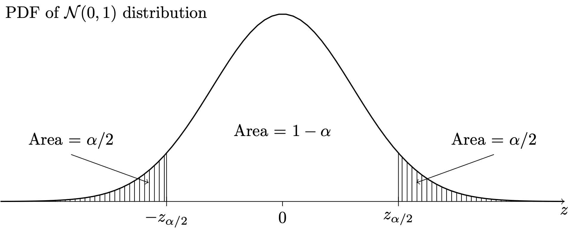
More generally, for any \(\alpha \in (0,1)\), we consider the construction of \((1-\alpha)100\%\) confidence intervals, where the value \(\alpha\) is the probability that our confidence interval will not contain \(\mu\). For a \(95\%\) confidence interval, the corresponding value of \(\alpha\) is \(0.05\). We refer to \(1-\alpha\) as the confidence level of the confidence interval. To give a general expression for a \((1-\alpha)100\%\) confidence interval, let \(z_{\alpha/2}\) denote the value such that \(P(Z > z_{\alpha/2}) = \alpha/2\), where \(Z \sim \mathcal{N}(0,1)\), as depicted here:
Figure 27.1: Depiction of upper quantile \(z_{\alpha/2}\).
The above is a depiction of what is called upper quantile notation. We call \(z_{\alpha/2}\) the upper\(\alpha/2\) quantile of the \(\mathcal{N}(0,1)\) distribution because there is area \(\alpha/2\) to the right of this value under the \(\mathcal{N}(0,1)\) PDF. Because the normal distributions are symmetric, the ordinary \(\alpha/2\) quantile is equal to \(-z_{\alpha/2}\), that is, it is the reflection of the upper \(\alpha/2\) quantile across the origin.
Then we have the following result:
Proposition 27.1 (Confidence interval for normal mean) For a random sample \(X_1,\dots,X_n \overset{\text{ind}}{\sim}\mathcal{N}(\mu,\sigma^2)\) with \(\sigma\) known, for any \(\alpha \in (0,1)\) the interval with endpoints \[
\bar X_n \pm z_{\alpha/2} \frac{\sigma}{\sqrt{n}}
\] will contain \(\mu\) with probability \(1-\alpha\).
We are very often interested in building confidence intervals at the \(0.90\), \(0.95\), or \(0.99\) confidence levels, for which Figure 14.5 depicts the necessary quantiles, \(z_{0.05} = 1.645\), \(z_{0.025} = 1.96\), and \(z_{0.005} = 2.576\), respectively, of the standard Normal distribution. Note that these quantities govern the width of the confidence interval, such that higher confidence corresponds to greater width.
Note that the confidence interval with endpoints given in Proposition 27.1 is constructed by adding and subtracting the same amount \(z_{\alpha/2}\sigma/\sqrt{n}\) to and from the sample mean \(\bar X_n\). When a confidence interval is constructed in this way, we will refer to the amount added and subtracted as the margin of error. Thus the width of such a confidence interval is two times the margin of error. Later on, in Chapter 32, we will consider the problem of selecting a sample size \(n\) in order to ensure that a confidence interval has a margin of error no larger than some desired bound.
Since the recipes for the construction of these intervals guarantees that they will contain the true value of \(\mu\) with probability \(1-\alpha\), we typically interpret our confidence intervals by saying, “we are \((1-\alpha)100\%\) confident that the true mean lies in this interval”.
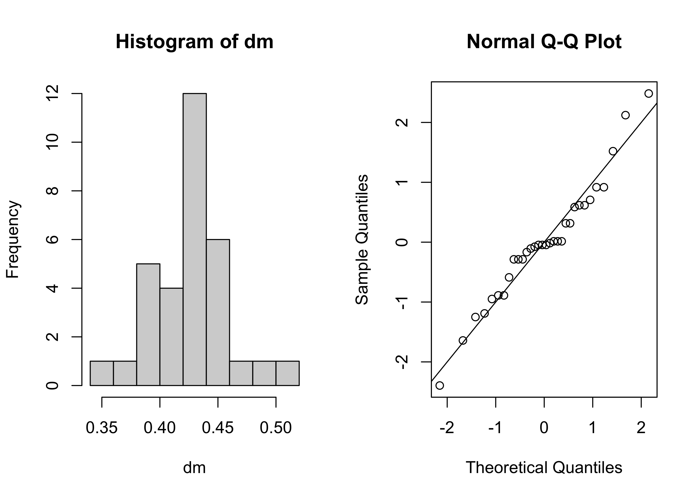
Example 27.1 (Confidence interval for mean acorn diameter) Suppose we wish to construct a 95% confidence interval for the mean diameter of live oak acorns using the data from Example 17.3. Based on the histogram and normal QQ plot shown below, it appears safe to assume that the diameters follow a normal distribution. Now, we do not know the value of \(\sigma\), but let’s use \(\sigma = 0.035\) (which is close to the value of the sample standard deviation \(S_n\) for these data) for constructing the interval.
Figure 27.2: Histogram and Normal QQ plot of live oak acorn diameters
The sample mean is \(\bar X_n = 0.43\) based on a sample of size \(n = 32\). With \(\alpha = 0.05\) we have \(z_{\alpha/2} = 1.96\). We thus obtain the 95% confidence interval \[
0.43 \pm 1.96 \frac{0.035}{\sqrt{32}} = [0.417, 0.442].
\] We would interpret this interval by saying, “We are 95% confident the mean diameter of live oak acorns is between \(0.417\) and \(0.442\).”
In order to build a \(99\%\) confidence interval for the mean diameter of live oak acorns, we set \(\alpha = 0.01\).
Then we obtain \(z_{\alpha/2} = 2.576\) and the 99% confidence interval becomes \[
0.43 \pm 2.576 \frac{0.035}{\sqrt{32}} = [0.414, 0.445].
\] We would interpret this interval by saying, “We are 99% confident the mean diameter of live oak acorns is between \(0.414\) and \(0.445\).”
Note that the \(99\%\) confidence interval is wider than the \(95\%\) confidence interval.
Exercise 27.1 (Confidence interval for the mean in golden ratio example) Regarding the values in the golden ratio data set as a random sample from a normal distribution with unknown mean \(\mu\) and standard deviation \(\sigma = 0.15\), construct a confidence interval for \(\mu\) at these confidence levels:
Note that Example 27.1 and Exercise 28.1 depended on knowledge of the population standard deviation \(\sigma\). Later on we will learn how to construct a confidence interval for \(\mu\) when \(\sigma\) is replaced by its sample counterpart \(S_n\).
The \(90\%\) confidence interval is given by \[
\bar X_n \pm 1.645 \frac{\sigma}{\sqrt{n}} = 1.56 \pm 1.645 \frac{0.15}{\sqrt{27}} = [1.513,1.607]
\]↩︎
The \(95\%\) confidence interval is given by \[
\bar X_n \pm 1.96 \frac{\sigma}{\sqrt{n}} = 1.56 \pm 1.96 \frac{0.15}{\sqrt{27}} = [1.503,1.617]
\]↩︎
The \(99\%\) confidence interval is given by \[
\bar X_n \pm 2.576 \frac{\sigma}{\sqrt{n}} = 1.56 \pm 2.576 \frac{0.15}{\sqrt{27}} = [1.486,1.634]
\]↩︎
This corresponds to \(\alpha = 0.02\), so that \(z_{\alpha/2} = z_{0.01} = 2.33\) (See the \(Z\) table in Chapter 46). \[
\bar X_n \pm 2.33 \frac{\sigma}{\sqrt{n}} = 1.56 \pm 2.33 \frac{0.15}{\sqrt{27}} = [1.493,1.627]
\]↩︎