ft <- c(2.5692,2.5936,2.6190,2.6320,2.6345,
        2.6602,2.6708,2.6804,2.6850,2.7049,
        2.7111,2.8034,2.8300,3.0639,3.1489,
3.2411,3.5701,3.9686,4.1220)17 The random sample
$$
$$
What we have been building up to so far is how to learn from data about the process which generated the data or about the population from which the data were drawn. However, we have not really encountered “data” yet. Our first (carefully controlled) encounter with data will be a study of what statisticians call a random sample. Imagine reaching into a population and selecting some of its members at random and measuring something about them or subjecting them to some experimental conditions and then measuring something about them. What results is a set of measurements such that each measurement i) can take more than one possible value, ii) must take a value belonging to a known set of values, and iii) takes a value which cannot be known in advance. In short, what results is a collection of random variables.
A random sample can be thought of as a set of values resulting from selecting some members of a population and taking measurements on them, possibly after subjecting them to some experimental conditions. Throughout, we will let \(n\) denote the number of values in the random sample, which we will refer to as the sample size. Formally, we define a random sample as follows:
Definition 17.1 (Random sample) A set of independent identically distributed random variables \(X_1,\dots,X_n\) is called a random sample of size \(n\).
We must admit that in the above definition we have used some terms that have not been defined yet. The first is independent. Even though we did define independence for two events \(A\) and \(B\), where we said \(A\) and \(B\) are independent if \(P(A \cap B) = P(A)P(B)\), and beyond this, we defined what it means for a collection of events to be mutually independent, we have not stated what we mean when we say that two random variables, or a set of more than two random variables, are independent. So, what is meant by the word “independence” in the above definition? Essentially, we say that two random variables \(X\) and \(Y\) are independent if the value of one does not effect the value of the other. To connect this to our definition of independence between two events, we can say that if random variables \(X\) and \(Y\) are independent, then we will have \[ P( X \in A \cap Y \in B) = P(X \in A) P(Y \in B) \] for all pairs of sets \(A\) and \(B\) which are subsets of the real numbers \(\mathbb{R}\).
The other new term appearing in Definition 17.1 is the phrase identically distributed. We say that two random variables \(X\) and \(Y\) are identically distributed if they have the same probability distribution. One way of expressing this is to say that \(X\) and \(Y\) have the same cumulative distribution function (CDF).
So, a random sample of size \(n\) is a set of random variables \(X_1,\dots,X_n\) such that i) the value of any one of them does not affect the value of any other one and ii) they all have the same probability distribution. This definition of a random sample is motivated by the oft-run experiment of drawing from a large population a certain number of members and measuring something on them; if the population is large enough, the draws can be considered independent (see the discussion on drawing with versus without replacement in Chapter 12). Moreover, since all the draws come from the same population, we can assume that all the measurements are realizations from a common distribution. Hereafter we will sometimes refer to the distribution shared by all the random variables in a random sample as the population distribution.
We may think of the random sample \(X_1,\dots,X_n\) as the values in a very simple data set. Here is an example:
Example 17.1 (Pinewood derby times) Several girls assembled and decorated pinewood derby cars and raced them, letting the cars roll down a ramp from a fixed starting point and timing (with a pretty sophisticated electronic timing system) how long it took them to cross a finish line. The finishing times are read into R in the code below.
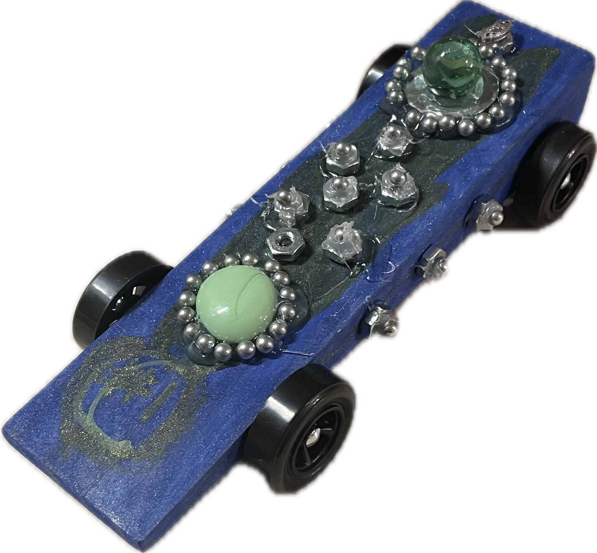
The R code below stores the observed values in a vector.
In the pinewood derby car example, an experiment is run: tell some young girls to assemble and decorate pinewood derby cars and race them, recording the finishing times. Now, do these measurements constitute a random sample? Perhaps they do, and perhaps they do not. Let’s consider whether the finishing times are independent. I know for a fact (being the father of two participants) that there was at least one pair of sisters in the competition, who more than likely (in fact) worked simultaneously and in close proximity to each other while assembling and decorating their cars. There may have been discussion between them, or a tip they both recieved from mom or dad, which could have lead them to use similar strategies of assembly and weighting, which may in the end have caused the finishing times of their cars to be similar. Yet it may be that the dependence induced in their finishing times by all of this may be slight enough to be negligible. As for whether the finishing times represent realizations of identically distributed random variables, it seems reasonable by the following: Even though each girl may have a unique decoration style and assembly strategy, if a girl is selected at random and the finishing time of her pinewood derby car is recorded, we can regard this finishing time as a draw from some distribution; and the collection of finishing times is a collection of draws from this same distribution. So, in spite of some possibility of non-independence, we will hereafter treat the pinewood derby car finishing times as a random sample.
Here is another example of a random sample which we will use.
Example 17.2 (Golden ratio data) Each in a class of twenty-seven students was asked to measure the distances \(A\) and \(B\) depicted below on his or her left hand and then to compute the ratio \(B/A\) of the distances.
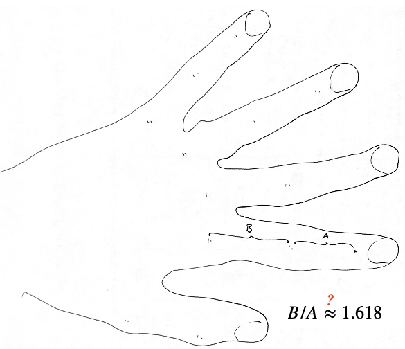
The R code below stores the observed values in a vector.
gr <- c(1.66, 1.61, 1.62, 1.69, 1.58, 1.43, 1.66,
        1.69, 1.58, 1.20, 1.52, 1.60, 1.55, 1.67,
        1.77, 1.50, 1.64, 1.54, 1.40, 1.36, 1.50,
        1.40, 1.35, 1.48, 1.64, 1.91, 1.70)
The instructor of the twenty-seven students was keenly interested in testing whether the average value of the ratio \(B/A\) was equal to the fabled golden ratio \((1 + \sqrt{5})/2\), which is \(1.618\) after rounding.
Example 17.3 (Live oak acorns) The lengths and diameters of thirty-two live oak acorns were measured using a pair of calipers.
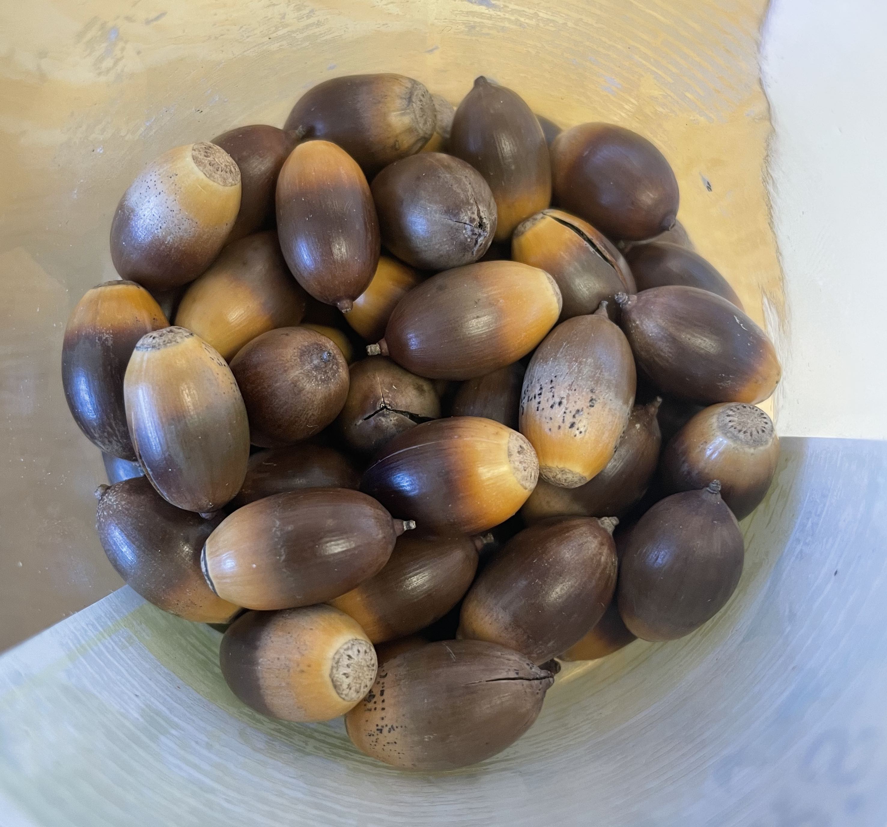
The code below reads the observed lengths and diameters into R.
# diameters
dm <- c(0.375,0.428,0.39,0.388,0.42,0.43,
        0.42,0.35,0.44,0.45,0.43,0.50,0.48,0.46,
        0.429,0.427,0.424,0.512,0.428,0.426,0.43,
        0.4,0.46,0.44,0.40,0.45,0.41,0.398,0.42,
        0.453,0.449,0.428)

# lengths
ln <- c(0.710,0.75,0.665,0.658,0.651,0.791,0.740,
        0.750,0.790,0.810,0.72,0.71,0.79,0.72,0.748,
        0.734,0.746,0.735,0.851,0.746,0.73,0.75,0.81,
        0.76,0.725,0.735,0.71,0.712,0.755,0.787,
        0.776,0.748)
Example 17.4 (Pallet weights) At Gregory’s Asparagus Farm each pallet on which lugs of asparagus are transported from the field into the barn is weighed in order that the net weight of the harvested asparagus (total weight minus the weight of the lugs–each weighing 3 lbs—minus the weight of the pallet) on each pallet can be recorded.
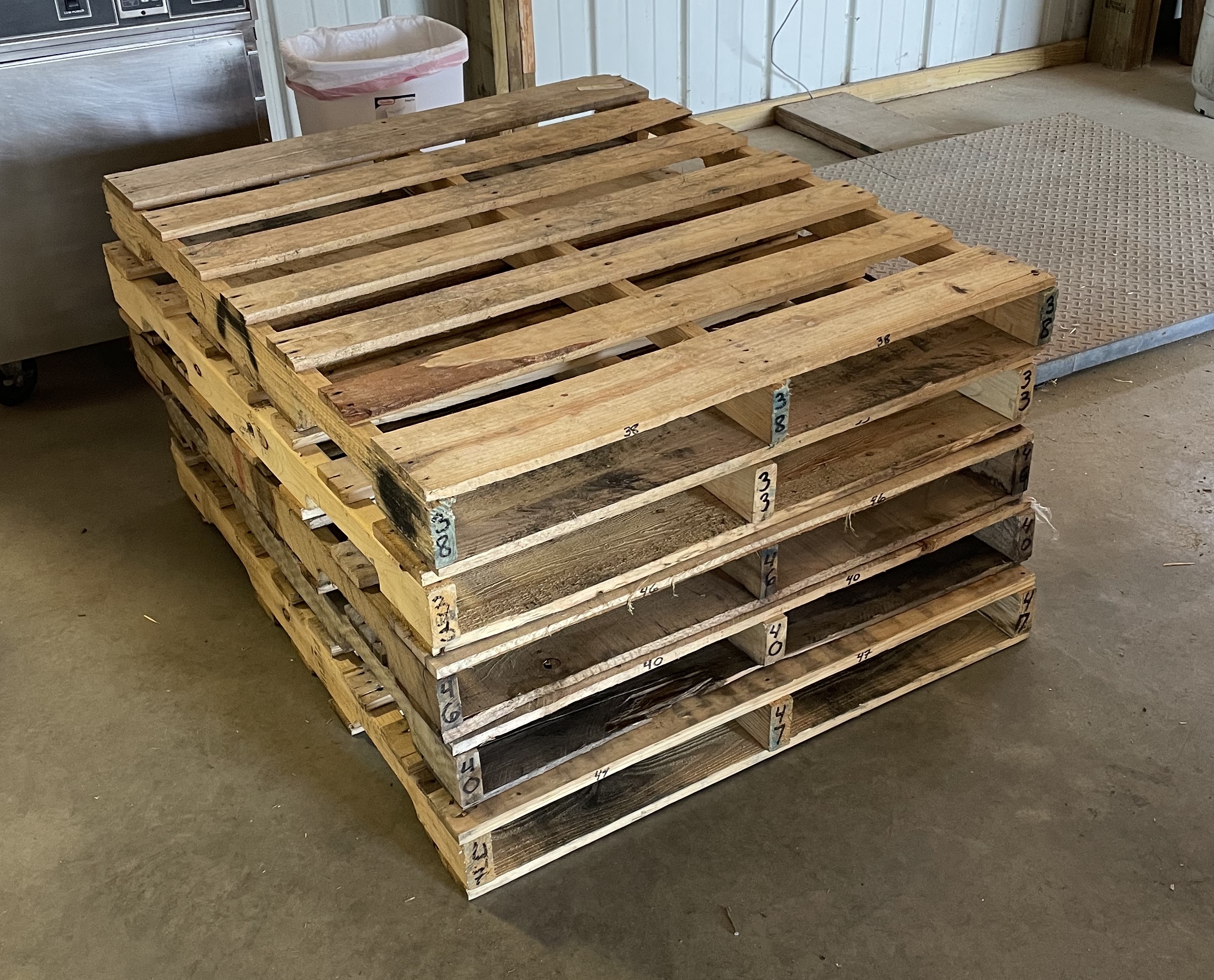
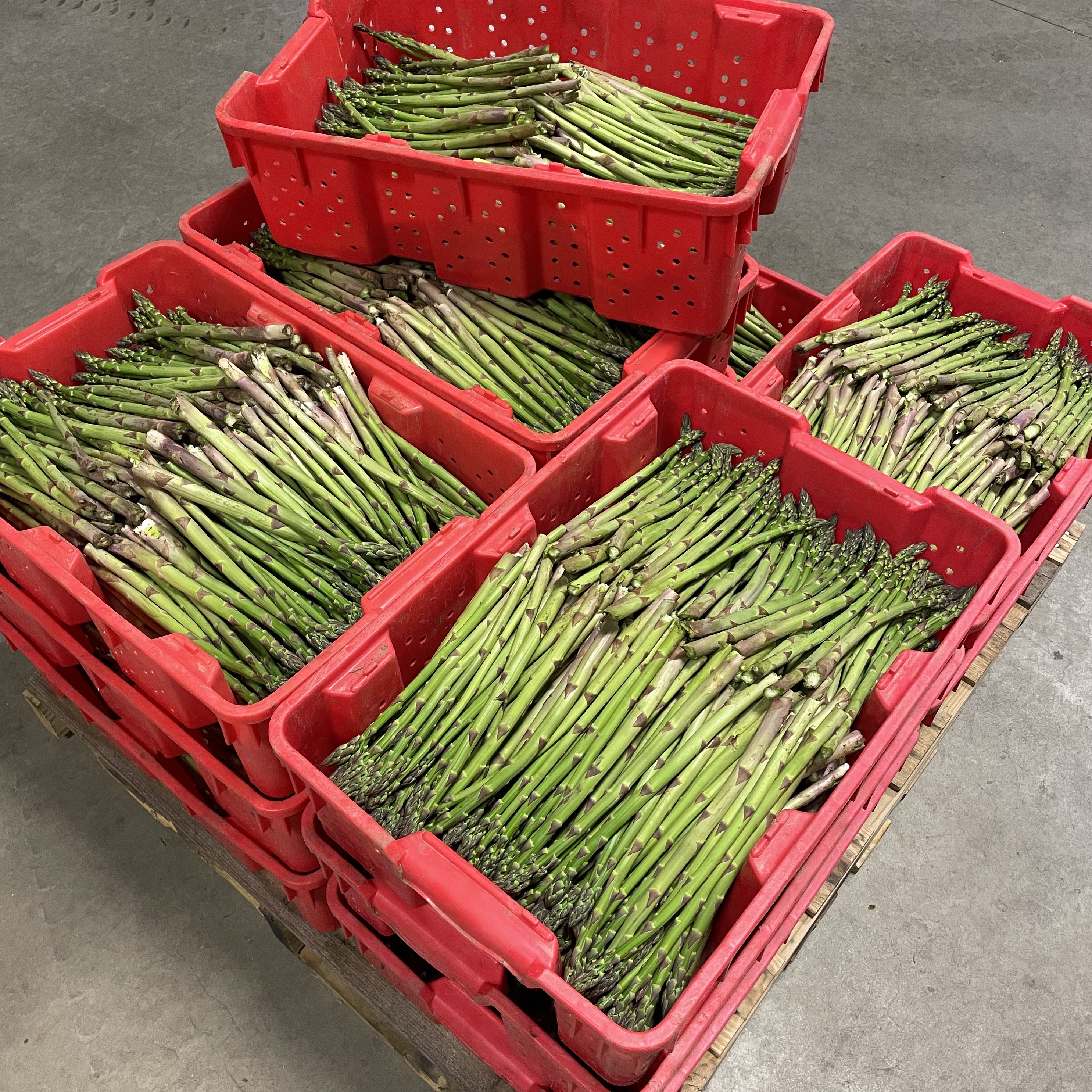
The weights of thirty-nine pallets used at Gregory’s Asparagus Far are read into R below:
wt <- c(41,34,40,44,33,42,52,38,32,31,31,35,
        39,44,42,42,35,33,40,48,51,32,41,35,
        38,48,37,35,42,41,40,47,40,46,33,38,
        51,39,40)
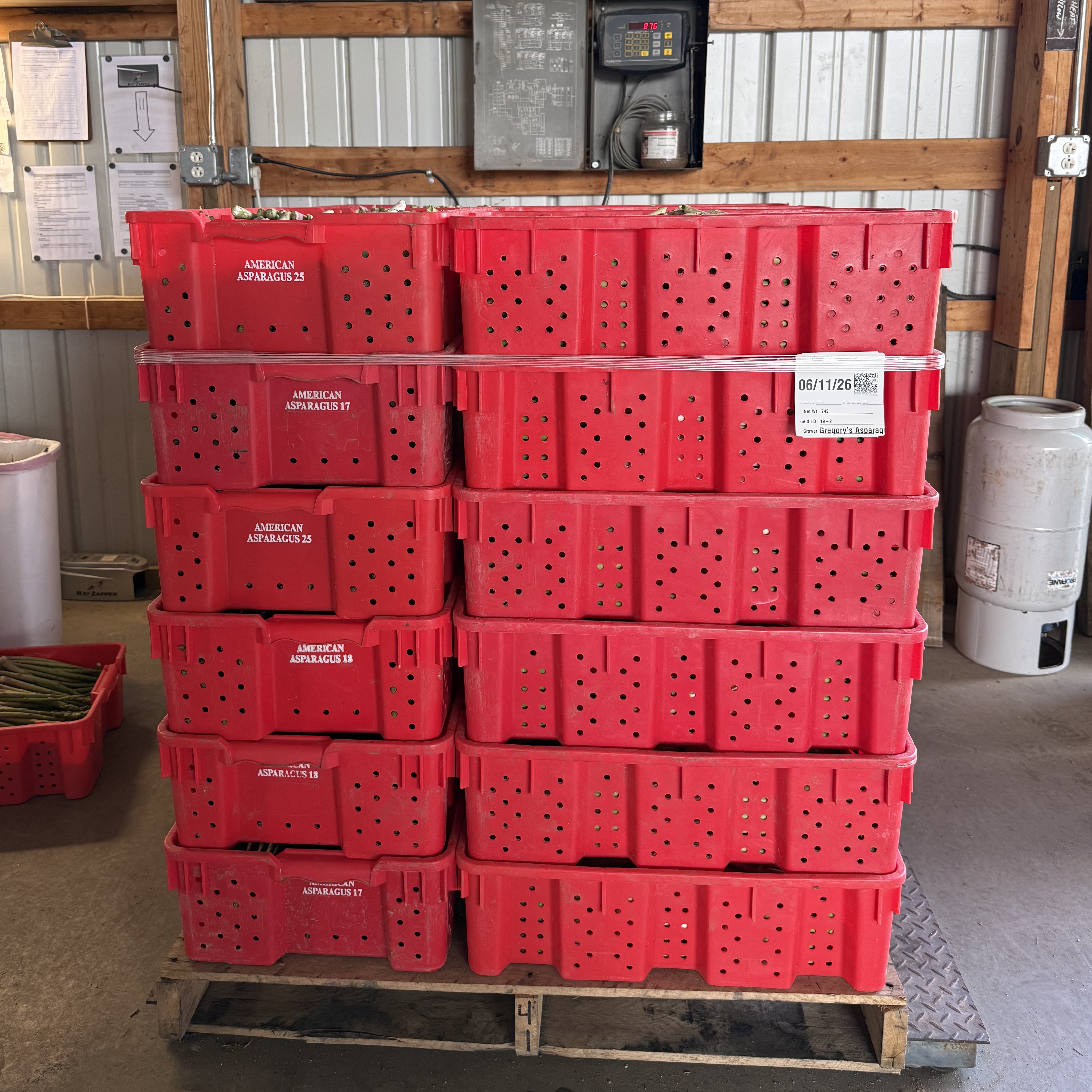
The distributor to whom Gregory’s Asparagus Farm sells its asparagus treats every pallet as though it weighed \(45\) pounds (a tag is attached to each out-going pallet which shows the net asparagus weight obtained under this assumption), as shown below. One may wonder if this is a good approximation to the weight of a pallet.
We may hereafter write \(X_1,\dots,X_n \overset{\text{ind}}{\sim}F\) to express that \(X_1,\dots,X_n\) are a random sample from a population with distribution \(F\). Often there are features of \(F\) that are unknown to us, and the goal of drawing the random sample \(X_1,\dots,X_n\) is to learn about these unknown features of \(F\). In particular, we will next consider how we can learn about the expected value of a random variable with distribution \(F\), which we may refer to as the population mean.