We’ll continue using the Pandas package for everything here.
Let’s read in the finisher data from the Table Rock 50k races in 2023 and 2024, which can be downloaded from here. The code below shows how we can do this:
import pandas as pddr ='/Users/karlgregory/Library/CloudStorage/OneDrive-UniversityofSouthCarolina/myBooks/compstat/data/'trcols = ['NA','Place','First','Last','City','State','Age','Division','DP','Time','Rank']tr23 = pd.read_table( dr +'tr50k_2023.txt', header =None, names = trcols, usecols =range(1,len(trcols)))tr24 = pd.read_table( dr +'tr50k_2024.txt', header =None, names = trcols, usecols =range(1,len(trcols)))tr24
Place
First
Last
City
State
Age
Division
DP
Time
Rank
0
1
Drew
Marshall
Charlotte
NC
30
M
1
4:15:08
93.78
1
2
Brent
Bookwalter
Montreat
NC
40
M
2
4:18:06
99.61
2
3
Devon
Brodmyer
Brevard
NC
22
M
3
4:42:09
93.33
3
4
Alan
Garvick
Leicester
NC
33
M
4
4:54:52
86.52
4
5
Jonathan
Keller
Woodruff
SC
27
M
5
4:57:10
85.85
...
...
...
...
...
...
...
...
...
...
...
200
201
Jessica
Jasinski
LINCOLNTON
NC
35
F
44
10:12:28
62.33
201
202
Matt
Kirchner
Atlanta
GA
41
M
158
10:12:28
51.43
202
203
Rick
Gray
Johnson City
TN
63
M
159
10:18:03
64.00
203
204
Kimber
Jones
Mars Hill
NC
33
F
45
10:24:42
56.73
204
205
Brandon
King
Weaverville
NC
36
M
160
10:24:44
68.37
205 rows × 10 columns
In R, to read names like O’something, we had to specify that ' should not be interpreted as a quoting character. The Pandas read_table function uses " by default, so our Irish names got read in okay this time.
ir = tr24['Last'].str.match(".*['].*") # any names with an apostrophe?tr24[ir]
Place
First
Last
City
State
Age
Division
DP
Time
Rank
32
33
Jack
O'Hara
Asheville
NC
28
M
30
6:09:57
68.96
41
42
Collin
O'Berry
Asheville
NC
39
M
39
6:29:01
73.81
Merging data sets
Let’s make a new data set containing, for each runner who participated in both the 2023 and 2024 Table Rock 50k races, the finishing times in both years. We use the merge function in the Pandas library.
You can do left joins and right joins with the merge function in Pandas as well. Consult the help file!
Concatenating data sets
Let’s read the data in from all the years, 2011 through 2024, using a loop, combining all the data into one large data frame. These data files can be downloaded from here.
li =list() # make a list of data frames to concatenate into one big onefor i inrange(11,25):file= dr +'tr50k_20'+str(i) +'.txt' tryr = pd.read_table( file, header =None, names = trcols, usecols =range(1,len(trcols))) tryr['Year'] ='20'+str(i) li.append(tryr) # append data frame to the list of data framestr = pd.concat(li)tr
Place
First
Last
City
State
Age
Division
DP
Time
Rank
Year
0
1
Wes
Kessenich
Waxhaw
NC
49
M
1
4:23:08
93.77
2011
1
2
Matt
Broughton
Sherrills Ford
NC
45
M
2
4:23:23
92.79
2011
2
3
Dwight
Winters
Morganton
NC
35
M
3
4:47:02
95.84
2011
3
4
Chris
Squires
Raleigh
NC
46
M
4
4:57:16
79.09
2011
4
5
Tammy
Tribett
Manassas
VA
39
F
1
4:59:00
75.58
2011
...
...
...
...
...
...
...
...
...
...
...
...
200
201
Jessica
Jasinski
LINCOLNTON
NC
35
F
44
10:12:28
62.33
2024
201
202
Matt
Kirchner
Atlanta
GA
41
M
158
10:12:28
51.43
2024
202
203
Rick
Gray
Johnson City
TN
63
M
159
10:18:03
64.00
2024
203
204
Kimber
Jones
Mars Hill
NC
33
F
45
10:24:42
56.73
2024
204
205
Brandon
King
Weaverville
NC
36
M
160
10:24:44
68.37
2024
2012 rows × 11 columns
Aggregating data
Let’s work towards getting the average time in each division for each year of the race. First we’ll need to convert the times to seconds, because right now they are just character strings. Below we define a function to make the conversion and then add a new column to the data set containing the columns in seconds.
def secs(ch): ch2 = ch.replace("`","") # for a tie, the character "`" is added, which we need to remove h, m, s = ch2.split(":") # split a character into multiple strings based on a splitting characterreturnint(h)*3600+int(m) *60+int(s) # can just put return in front of an expressiontr['Seconds'] = tr['Time'].map(secs)tr
Place
First
Last
City
State
Age
Division
DP
Time
Rank
Year
Seconds
0
1
Wes
Kessenich
Waxhaw
NC
49
M
1
4:23:08
93.77
2011
15788
1
2
Matt
Broughton
Sherrills Ford
NC
45
M
2
4:23:23
92.79
2011
15803
2
3
Dwight
Winters
Morganton
NC
35
M
3
4:47:02
95.84
2011
17222
3
4
Chris
Squires
Raleigh
NC
46
M
4
4:57:16
79.09
2011
17836
4
5
Tammy
Tribett
Manassas
VA
39
F
1
4:59:00
75.58
2011
17940
...
...
...
...
...
...
...
...
...
...
...
...
...
200
201
Jessica
Jasinski
LINCOLNTON
NC
35
F
44
10:12:28
62.33
2024
36748
201
202
Matt
Kirchner
Atlanta
GA
41
M
158
10:12:28
51.43
2024
36748
202
203
Rick
Gray
Johnson City
TN
63
M
159
10:18:03
64.00
2024
37083
203
204
Kimber
Jones
Mars Hill
NC
33
F
45
10:24:42
56.73
2024
37482
204
205
Brandon
King
Weaverville
NC
36
M
160
10:24:44
68.37
2024
37484
2012 rows × 12 columns
Here we define a function which will convert a number of seconds into a time in the form hh:mm:ss:
import timedef secs2time(x):return time.strftime("%H:%M:%S",time.gmtime(x)) # number of seconds from 00:00:00, Jan 1, 1970 GMT, re-express as hh:mm:ss
Now we apply the function defined above to the seconds series of the data frame using map:
tm = tr.pivot_table( values ='Seconds', index = ['Year','Division'], aggfunc = {'Seconds' : 'mean'})tm['Ave. Time'] = tm.Seconds.map(secs2time) # use .map to apply the functiontm.drop('Seconds', axis =1) # get rid of the 'Seconds' series
Ave. Time
Year
Division
2011
F
06:42:20
M
06:10:06
2012
F
06:24:39
M
06:04:34
2013
F
06:38:18
M
05:47:18
2014
F
07:44:31
M
07:51:12
2015
F
08:12:44
M
07:45:11
2016
F
07:48:02
M
07:49:02
2017
F
08:07:43
M
07:39:59
2018
F
08:39:39
M
08:02:19
2019
F
07:57:04
M
07:26:02
2020
F
08:08:10
M
06:59:01
2021
F
08:05:19
M
07:24:56
2022
F
07:53:16
M
07:20:23
2023
F
08:01:09
M
07:07:56
2024
F
08:09:41
M
07:36:25
age = tr.pivot_table( values ='Age', index = ['Year','Division'], aggfunc = {'Age' : ['min','median','max']}) # min, median, and max are recognized built-in functionsage
Note that with pivot tables, Pandas introduces what is called a multi-index, which is just a hierarchical index. In this example we have the division within the year, so to access a row of the above table, we need to give both the year and the division as a tuple:
tr_pctl.loc[('2011','M'),] # access rows of this with a tuple
90th percentile    18184.0
95th percentile    17283.4
Best               15788.0
Name: (2011, M), dtype: float64
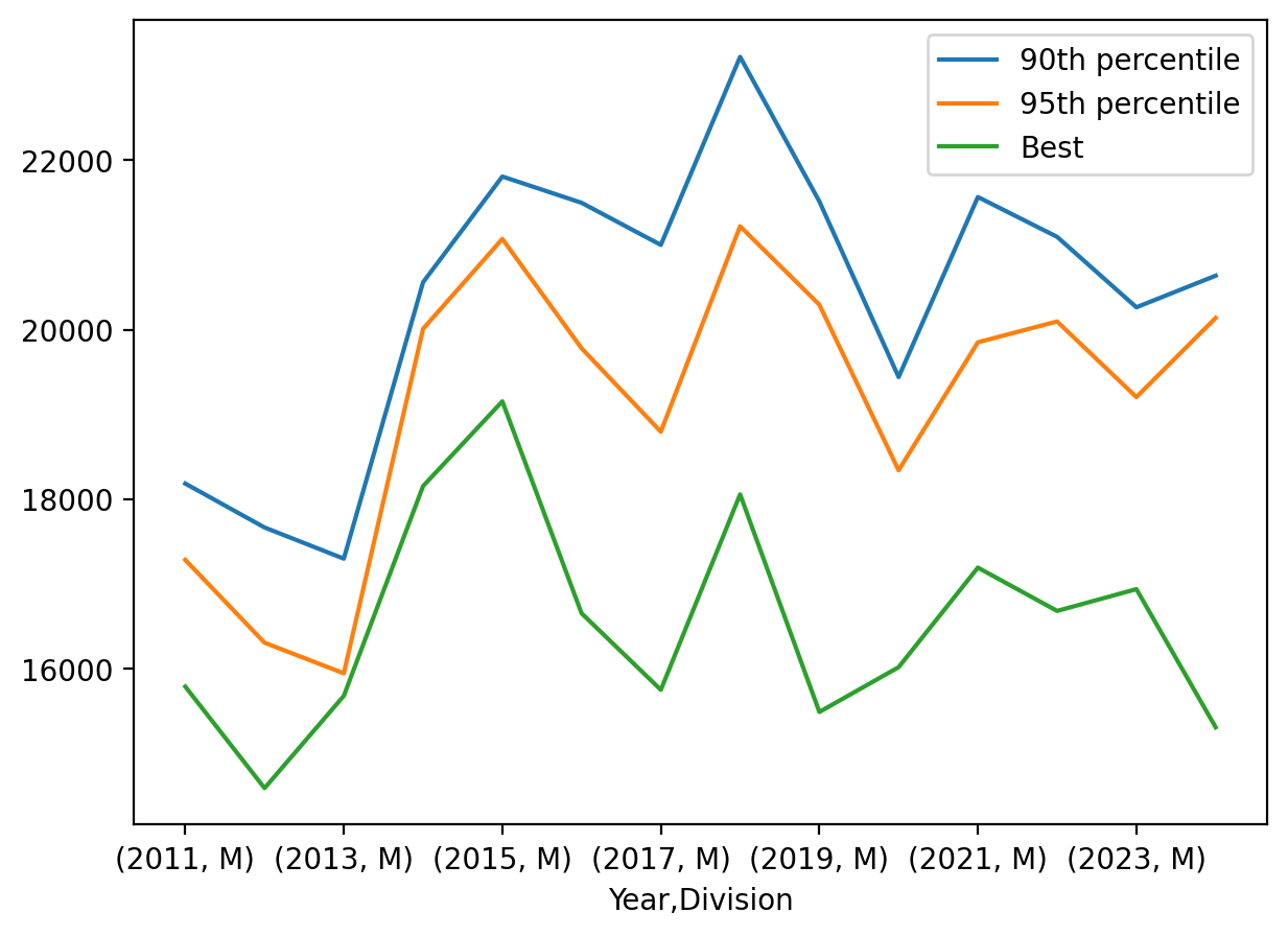
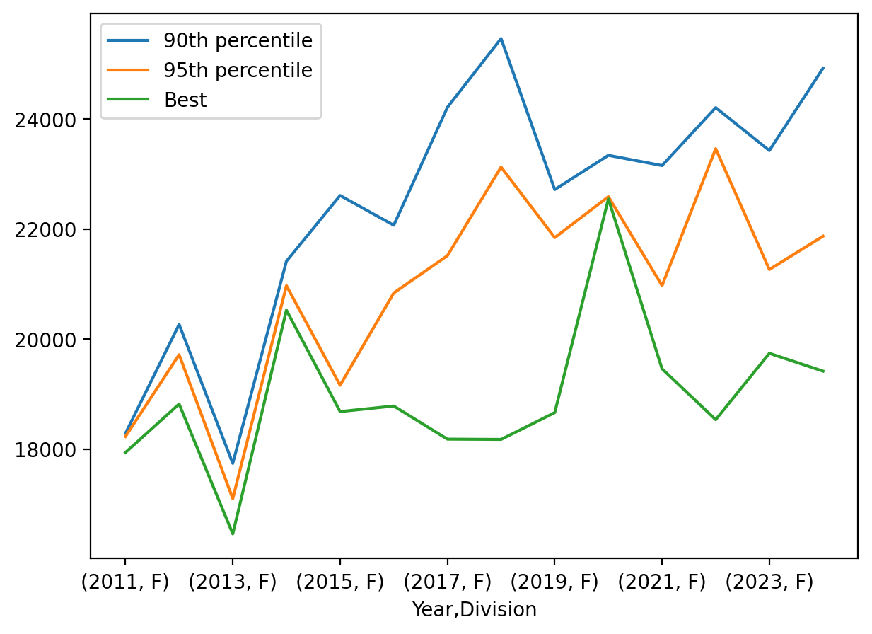
Let’s plot these quantiles over the years of the Table Rock 50k for each division.
tr_pctl_M = tr_pctl.loc[(slice(None),'M'),] # keep all rows of the first index
tr_pctl_F = tr_pctl.loc[(slice(None),'F'),] # keep all rows of the first index
tr_pctl_M.plot()tr_pctl_F.plot()
If we want to get rid of the multi-indices, we can do so using the resent_index method as below.
tr_pctl_nomulti = tr_pctl.reset_index(None) # the pivot_table creates multi-indexes that you can get rid of with .reset_index(None)tr_pctl_nomulti
Year
Division
90th percentile
95th percentile
Best
0
2011
F
18287.0
18231.00
17940
1
2011
M
18184.0
17283.40
15788
2
2012
F
20267.9
19718.00
18821
3
2012
M
17665.6
16306.20
14590
4
2013
F
17743.0
17102.50
16462
5
2013
M
17297.8
15944.70
15679
6
2014
F
21416.9
20971.95
20527
7
2014
M
20559.3
20009.55
18154
8
2015
F
22611.2
19162.80
18684
9
2015
M
21807.1
21071.15
19154
10
2016
F
22070.6
20839.60
18785
11
2016
M
21497.1
19780.10
16653
12
2017
F
24213.4
21517.30
18183
13
2017
M
21000.0
18796.20
15750
14
2018
F
25463.9
23127.50
18178
15
2018
M
23219.0
21220.00
18056
16
2019
F
22719.1
21845.65
18665
17
2019
M
21513.4
20295.00
15489
18
2020
F
23341.6
22589.60
22548
19
2020
M
19441.0
18340.80
16017
20
2021
F
23155.4
20972.40
19461
21
2021
M
21565.4
19851.10
17192
22
2022
F
24208.1
23461.45
18537
23
2022
M
21095.0
20096.75
16681
24
2023
F
23428.1
21265.85
19743
25
2023
M
20264.0
19204.80
16938
26
2024
F
24923.8
21871.20
19419
27
2024
M
20637.0
20138.25
15308
Just because, let’s convert the times in this table to durations represented as hh:mm:ss:
We can reshape a data set in “long” format to “wide” format with the pivot method for Pandas data frames. Here we make a data frame showing the finishing times of the first three finishers in the years 2011 to 2024.
pod = tr['Place'] <=3tr_pod = tr[pod]tr_pod.pivot(index ='Place', values ='Time', columns='Year')
Year
2011
2012
2013
2014
2015
2016
2017
2018
2019
2020
2021
2022
2023
2024
Place
1
4:23:08
4:03:10
4:21:19
5:02:34
5:11:24
4:37:33
4:22:30
5:00:56
4:18:09
4:26:57
4:46:32
4:38:01
4:42:18
4:15:08
2
4:23:23
4:31:35
4:22:00
5:23:32
5:19:14
4:52:18
4:41:06
5:01:33
5:01:42
4:34:21
4:47:37
4:51:39
4:46:22
4:18:06
3
4:47:02
4:31:51
4:34:22
5:34:01
5:20:16
4:54:49
4:54:47
5:02:58
5:07:24
4:49:28
4:50:14
5:08:57
4:47:12
4:42:09
Now let’s look at the top 3 places in each division in each year:
The wide_to_long function can be used to convert a data set in “wide” format to “long” format. To illustrate how to do this, let’s convert our wide dataset showing the times of the top three finishers in each division in each year back into long format. In order to do that, we will need to “flatten out” the multi-indices created in the pivot operation.