SQL in R

Author

Karl Gregory

Now that we know how to make some simple SQL queries, we consider how to import SQL-retrieved data into R so that we can make plot or do statistical analyses of the data. In this page we’ll learn how to store the results of SQL queries in R data frames.

Let’s continue working with the airlines database, accessible via the mdsr package:

library(mdsr) 
db <- dbConnect_scidb("airlines")

One way to store the result of an SQL queries in an R data frame is by using the R package DBI.

library(DBI) # first time run install.packages("DBI")

This package has the function dbGetQuery(), which returns a data frame from an SQL query. Here is an example of how it is used:

query <- "
SELECT faa, alt, lat, lon
FROM airports
WHERE alt > 5280
"

hap <- dbGetQuery(db, query)
head(hap)

  faa  alt      lat       lon
1 36U 5637 40.48181 -111.4288
2 4U9 6007 44.73575 -112.7200
3 A50 6145 38.87000 -104.4100
4 ABQ 5355 35.04022 -106.6092
5 ALS 7539 37.43500 -105.8667
6 APA 5883 39.57013 -104.8493

So we need to provide two arguments to the dbGetQuery() function: First, the database, and second, a text string containing a valid SQL query. The function executes the query and returns the result as an R data frame.

Make some maps

Now we can use the retrieved data in R: The code below makes a map of the United States of America using the R package maps and places dots at the locations of these airports.

library(maps) # first time run install.packages("maps")
map('state')
points(x = hap$lon, y = hap$lat, pch = 19)
text(x = hap$lon, y = hap$lat, labels = hap$faa, cex = .5, pos = 3)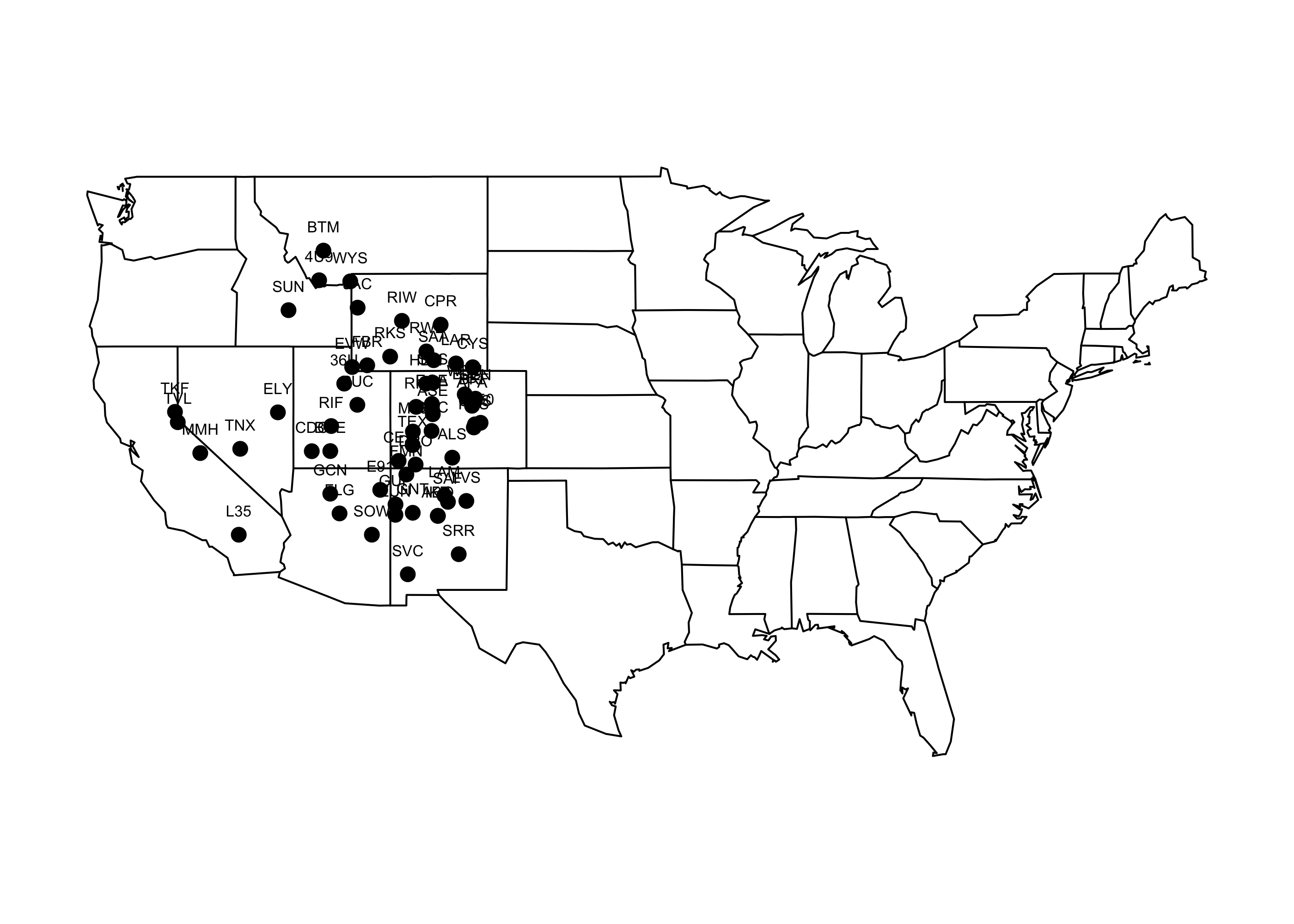

Now let’s find mile-high airports from which a flight to Miami (MIA) departed during 2013, keeping their longitude and latitude coordinates.

query <- "
SELECT f.origin, f.dest, a.alt, COUNT(*) numFlights, a.lon, a.lat
FROM flights AS f
JOIN airports AS a ON f.origin = a.faa
WHERE a.alt > 5280 AND f.year = '2013' AND f.dest = 'MIA'
GROUP BY f.origin
"

tomiami <- dbGetQuery(db,query)
tomiami

  origin dest  alt numFlights       lon      lat
1    DEN  MIA 5431        747 -104.6732 39.86166
2    EGE  MIA 6540        104 -106.9177 39.64256

Note, if we want a data frame in R to print nicely in a markdown document, we can use the kable() function from the R package knitr, as follows:

library(knitr)
kable(tomiami[,-c(3,5,6)], 
      col.names = c("Origin","Destination","Number of flights in 2013"))

Origin	Destination	Number of flights in 2013
DEN	MIA	747
EGE	MIA	104

Let’s get the longitude and latitude of the Miami airport too:

query <- "
SELECT faa, lon, lat
FROM airports
WHERE faa = 'MIA'
"

miami <- dbGetQuery(db,query)
miami

  faa       lon      lat
1 MIA -80.29056 25.79325

The code below makes a plot showing possible flight paths from the mile-high airports to the MIA airport. The code makes use of a function in the R package geosphere for computing the coordinates of a geodesic (shortest line between two points on a sphere) between these airports and MIA.

map('state')

points(x = tomiami$lon, y = tomiami$lat)
points(x = miami$lon, y = miami$lat)

text(x = tomiami$lon, 
     y = tomiami$lat, 
     labels = tomiami$origin, 
     pos = 3, 
     cex = .6)

text(x = miami$lon, 
     y = miami$lat, 
     labels = miami$faa, 
     pos = 3, 
     cex = .6)

library(geosphere) # gcIntermediate computes the geodesic between two (lon,lat) coordinates
geo1 <- gcIntermediate(p1 = c(tomiami$lon[1],tomiami$lat[1]),
                       p2 = c(miami$lon,miami$lat))
geo2 <- gcIntermediate(p1 = c(tomiami$lon[2],tomiami$lat[2]),
                       p2 = c(miami$lon,miami$lat))
lines(geo1)
lines(geo2)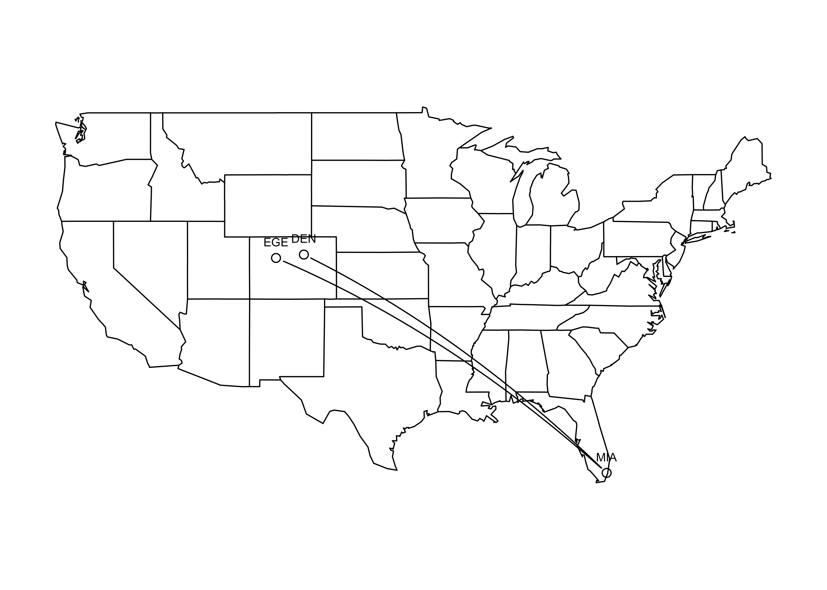

Plot number of departures over time

Below we obtain the number of departures from ATL every day:

query = "
  SELECT origin, COUNT(*) AS numDepartures, STR_TO_DATE(CONCAT(year,'/', month,'/', day),'%Y/%m/%d') AS theDate
  FROM flights
  WHERE origin = 'ATL'
  GROUP BY year, month, day
"

dep <- dbGetQuery(db, query)

Now we plot, for each weekday, the number of departures over 2013 – 2015:

wkdays <- c("Sunday","Monday","Tuesday","Wednesday","Thursday","Friday","Saturday")
wkdays_dep <- weekdays(dep$theDate)

plot(numDepartures ~ theDate, 
     data = dep,
     pch = NA, 
     bty = "l",
     ylab = "Number of departures from ATL",
     xlab = "Date") # make empty plot

for(j in 1:7){
  
  ind <- which(wkdays_dep == wkdays[j])
  lines(numDepartures ~ theDate, data = dep[ind,], col = j, lty = j)

}

legend("bottom",
       legend = c("Su","Mo","Tu","We","Th","Fr","Sa"),
       lty = 1:7, 
       col = 1:7, 
       horiz = T, 
       bty = "n")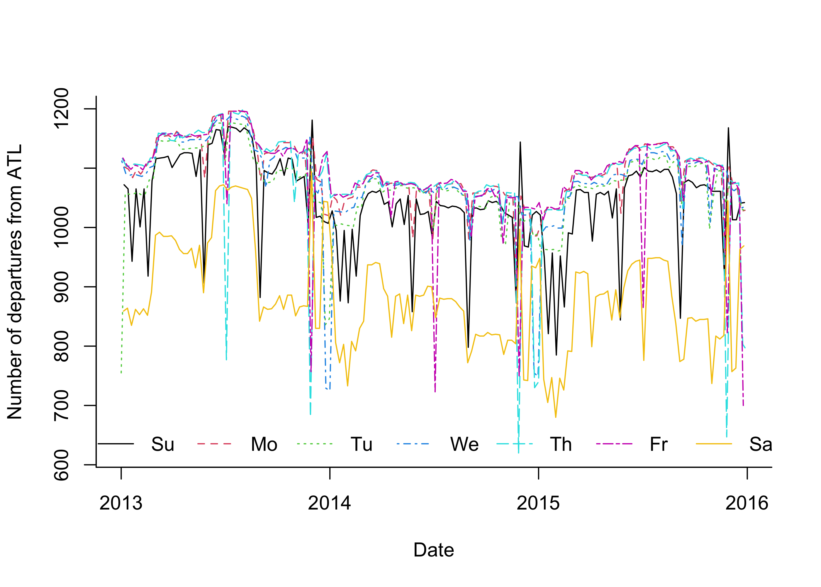

query <- "
SELECT distance
FROM flights
WHERE year = 2013 AND month = 1 AND day = 15
"

dist <- dbGetQuery(db,query)

hist(dist$distance,
     breaks = 50,
     main = 'Flight distances for all US domestic flights on Jan 15, 2013',
     xlab = 'Distance')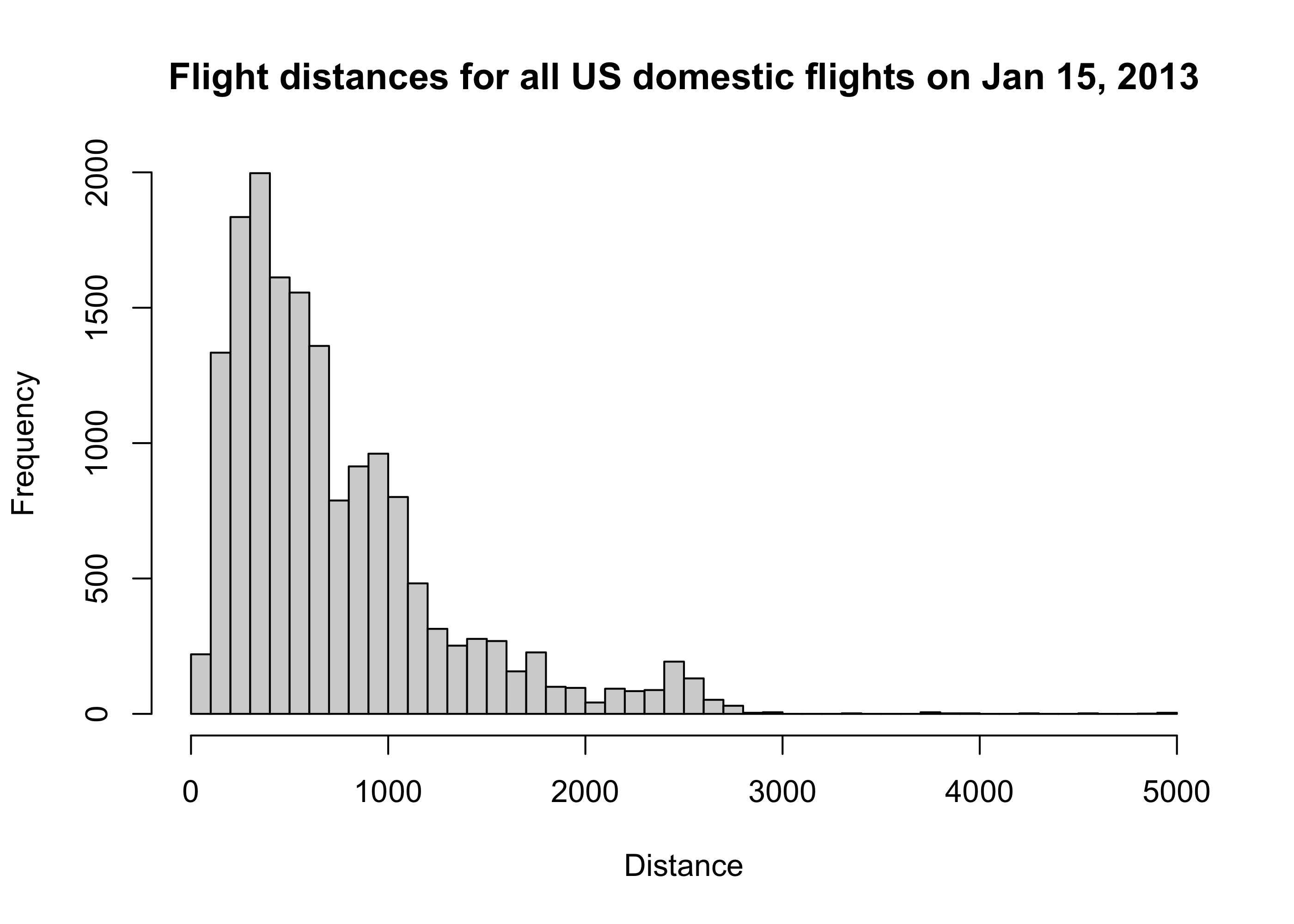

Let’s find out the origins and destination of these really long flights:

query <- "
SELECT f.distance, o.name AS origin, d.name AS destination
FROM flights as f
JOIN airports as o ON f.origin = o.faa
JOIN airports as d ON f.dest = d.faa
WHERE f.year = 2013 AND f.month = 1 AND f.day = 15 AND f.distance >= 3000
"

longflights <- dbGetQuery(db,query)

kable(longflights)

distance	origin	destination
4983	John F Kennedy Intl	Honolulu Intl
3904	George Bush Intercontinental	Honolulu Intl
4243	Chicago Ohare Intl	Honolulu Intl
4502	Hartsfield Jackson Atlanta Intl	Honolulu Intl
3784	Dallas Fort Worth Intl	Honolulu Intl
3711	Dallas Fort Worth Intl	Kahului
3365	Denver Intl	Honolulu Intl
3784	Dallas Fort Worth Intl	Honolulu Intl
4817	Washington Dulles Intl	Honolulu Intl
4963	Newark Liberty Intl	Honolulu Intl
4983	Honolulu Intl	John F Kennedy Intl
4502	Honolulu Intl	Hartsfield Jackson Atlanta Intl
3784	Honolulu Intl	Dallas Fort Worth Intl
3711	Kahului	Dallas Fort Worth Intl
3784	Honolulu Intl	Dallas Fort Worth Intl
4243	Honolulu Intl	Chicago Ohare Intl
3904	Honolulu Intl	George Bush Intercontinental
4963	Honolulu Intl	Newark Liberty Intl
3365	Honolulu Intl	Denver Intl