Below we read in each text file to a data frame with the brilliant and beautiful read.table() function. There is no “header” in this file giving the names of the columns, so if we want nice column names we have to provide them (otherwise they will be named V1, V2, and so on), which we can do with the col.names = option. We can specify the classes of the columns with the colClasses = option; with this option we can also specify which, if any, columns we don’t want read in:
columns <-c(NA,"Place","First","Last", "City", "State", "Age", "Division", "DP", "Time", "Rank")# put "NULL" if you want to skip a column! We don't want the first one.classes <-c("NULL", "numeric",rep("character",4),"numeric","character","numeric","character","numeric")tr50k_2023 <-read.table(file ="data/tr50k_2023.txt", sep ="\t", # data are tab separatedquote ="", # some apparently Irish folk ran this race, with names like O'Something. The "'" is used by default as a quote character, so this messed things up. Had to specify the option quote = "".col.names = columns,colClasses= classes)# read the 2024 data in the same waytr50k_2024 <-read.table(file ="data/tr50k_2024.txt", sep ="\t",quote ="", col.names = columns,colClasses= classes)
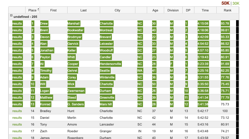
Since these are fairly large data frames, we may just want to see a small preview of their contents. We can use the head() function to print only the first several rows:
head(tr50k_2023)
  Place   First     Last      City State Age Division DP    Time  Rank
1     1   James Thompson Asheville    NC  39        M  1 4:42:18 93.55
2     2  Robbie    Harms  Fletcher    NC  30        M  2 4:46:22 87.05
3     3   Chris   Ingram Charlotte    NC  43        M  3 4:47:12 81.69
4     4    Alex    Black  Marshall    NC  33        M  4 4:56:19 77.94
5     5    Mark  Rebholz Charlotte    NC  33        M  5 4:56:44 88.10
6     6 William  Connell   Astoria    NY  40        M  6 4:57:45 86.15
head(tr50k_2024)
  Place    First       Last      City State Age Division DP    Time  Rank
1     1     Drew   Marshall Charlotte    NC  30        M  1 4:15:08 93.78
2     2    Brent Bookwalter  Montreat    NC  40        M  2 4:18:06 99.61
3     3    Devon   Brodmyer   Brevard    NC  22        M  3 4:42:09 93.33
4     4     Alan    Garvick Leicester    NC  33        M  4 4:54:52 86.52
5     5 Jonathan     Keller  Woodruff    SC  27        M  5 4:57:10 85.85
6     6   Peyton      Whitt   Candler    NC  23        M  6 5:19:43 80.91
Now, a handful of the long-distance runner types actually ran the Table Rock 50k in 2023 and 2024. Suppose we want to make a data set of just these runners, so we can compare their performances in the two years.
To achieve this we will use the merge() function. The merge function takes as arguments the two data sets as well as a by = argument which specifies which column or columns identify each unique record in the two data sets. The merge() function will return a new data frame containing the by = column (or columns) as well as all the other columns from each data frame; but the new data frame will include only records for identifiers appearing in both data sets. This is the default behavior of the merge() function: You get the intersection of the two data sets, which is the set of records with the identifier appearing in both. This is sometimes called an inner join. One can also specify the suffixes = option to change the way columns from the two data frame are renamed when they are brought into the new data frame.
       Last    First Place_23 Place_24 Time_23  Time_24
1     Corey     Adam       12        9 5:29:05  5:31:55
2   Cushman     Kati      133       64 7:55:59  6:59:52
3  Donoghue  Patrick       21       26 5:50:24  5:55:23
4      Ford     Ryan       67      107 6:50:58  7:54:12
5      Gray Michelle       34       47 6:17:49  6:48:08
6      Gray     Rick      186      203 9:58:03 10:18:03
7      Hall   Andrew       44       39 6:29:50  6:25:33
8  Hastings    Liana      108      157 7:33:00  8:41:13
9   Hinshaw     Jake       59       40 6:39:17  6:25:35
10   Jeffus    Tyson       48       32 6:32:04  6:07:53
11     Kira      Rio      141      127 8:01:30  8:13:46
12 McDowell      Amy      173      192 9:15:15  9:44:09
13   Merlin   Daniel       49       15 6:33:04  5:42:52
14   Newell  Timothy       94       55 7:20:10  6:55:19
15       Ng     Ivan       57       76 6:36:15  7:13:36
16  Nielsen    David       25       27 5:55:03  6:01:44
17     Pace   Travis       24       21 5:53:17  5:46:06
18    Peter   Bryson       47       45 6:31:10  6:44:51
19    Steed   Hunter       56       53 6:35:50  6:52:47
20    Steed  Matthew       27       12 5:57:55  5:41:34
21    Wells   Daniel      136      150 7:57:52  8:35:15
22    Wells  Spencer      137      154 7:57:55  8:38:07
23  Wingler    Jared       99       89 7:29:25  7:27:15
We see that 23 runners participated in both the 2023 and 2024 Table Rock 50k. Cool!
Another way to use the merge() function is, instead of keeping only the records in the intersection of the two data frames, to keep all the records from one or the other during the merge. Naming the arguments x = and y = such that the first data set is x and the second is y, we can set the option all.x = T so that all the records from the x data frame are kept. If we do this, we keep all the records in the x data set, even though there will be will be no corresponding identifier in the y data set for some of these. This results in the assignment of missing values to these records in the columns coming from the y data set. This is sometimes called a left outer join.
    Last    First Place_23      City_23 State_23 Age_23 Division_23 DP_23
1  Abreo   Justin      115 Fayetteville       NC     31           M   101
2 Adcock Jonathan      104       Stuart       VA     41           M    93
3 Adcock      Reb      153       Stuart       VA     43           F    27
4  Allen     Alex      160     Hoschton       GA     33           M   129
5  Annas     Matt      177    Morganton       NC     38           M   140
6  Annas   Torrey      176    Morganton       NC     37           F    37
  Time_23 Rank_23 Place_24 City_24 State_24 Age_24 Division_24 DP_24 Time_24
1 7:40:15   71.69       NA    <NA>     <NA>     NA        <NA>    NA    <NA>
2 7:31:44   69.70       NA    <NA>     <NA>     NA        <NA>    NA    <NA>
3 8:19:49   72.87       NA    <NA>     <NA>     NA        <NA>    NA    <NA>
4 8:34:22   51.70       NA    <NA>     <NA>     NA        <NA>    NA    <NA>
5 9:22:14   52.02       NA    <NA>     <NA>     NA        <NA>    NA    <NA>
6 9:22:13   59.13       NA    <NA>     <NA>     NA        <NA>    NA    <NA>
  Rank_24
1      NA
2      NA
3      NA
4      NA
5      NA
6      NA
We can likewise do a right outer join, which keeps all the records in the y data set.
      Last     First Place_23 City_23 State_23 Age_23 Division_23 DP_23 Time_23
1   Alford Nathaniel       NA    <NA>     <NA>     NA        <NA>    NA    <NA>
2    Amore      Tony       NA    <NA>     <NA>     NA        <NA>    NA    <NA>
3 Atkinson     James       NA    <NA>     <NA>     NA        <NA>    NA    <NA>
4    Baker  Patricia       NA    <NA>     <NA>     NA        <NA>    NA    <NA>
5  Barrett    Andrew       NA    <NA>     <NA>     NA        <NA>    NA    <NA>
6    Beard  Jennifer       NA    <NA>     <NA>     NA        <NA>    NA    <NA>
  Rank_23 Place_24         City_24 State_24 Age_24 Division_24 DP_24 Time_24
1      NA       41    Johnson City       TN     24           M    38 6:26:30
2      NA       16       Lancaster       SC     44           M    15 5:43:16
3      NA      140 Fort Eisenhower       GA     44           M   112 8:29:43
4      NA      152         Raleigh       NC     33           F    33 8:36:20
5      NA      169     Chapel Hill       NC     57           M   132 8:56:42
6      NA      103         Sanford       NC     42           F    18 7:49:28
  Rank_24
1   71.60
2   80.91
3   51.63
4   62.68
5   73.90
6   66.96
Stacking data sets
We may want to combine two data sets by simply stacking one on top of the other. This is possible when the data sets have the same columns. In our case, we would like to keep track of which records came from the 2023 data and which came from the 2024 data. The code below adds a column to each data set with entries giving the year, either 2023 or 2024. We can then use the rbind() function (we used it before to stack matrices) to stack the two data sets:
tr50k_2023$Year <-2023tr50k_2024$Year <-2024tr50k <-rbind(tr50k_2023,tr50k_2024) # here is the stacking with rbind()tr50k <-subset(tr50k,select =c("Place","Time","Last","First","Year")) # keep only certain columnshead(sort_by(tr50k,~Place)) # let's sort the data by place
    Place    Time       Last  First Year
1       1 4:42:18   Thompson  James 2023
188     1 4:15:08   Marshall   Drew 2024
2       2 4:46:22      Harms Robbie 2023
189     2 4:18:06 Bookwalter  Brent 2024
3       3 4:47:12     Ingram  Chris 2023
190     3 4:42:09   Brodmyer  Devon 2024
Reshaping a data set
Another way in which we might want to manipulate a data set is to “reshape” it. By “reshaping”, one typically means doing a long to wide or a wide to long transformation of the data set.
Long to wide
The tr50k data set contains all the Table Rock 50k data from the years 2023 and 2024, where the number of rows is equal to the total number of finishers of these two races. Suppose we would like construct a table for comparing the finishing times of the 1st-place finishers in the two years as well as the 2nd-place finishers in the two years and so on. That is, suppose we want a table where each row corresponds to a place and in each row we can see who finished at that place and with what finishing time in the year 2023 as well as in the year 2024.
We can achieve this with the reshape() function in R. This function was designed with longitudinal data in mind, which are data collected over time. Consider a “toy” experiment involving two subjects, where a response is measured on each subject at four observation times. The data might be presented in a table like this:
If we want instead to represent the data in a table having one row for each subject and four columns giving the four observations, we can obtain it with the reshape() function as follows:
wide <-reshape(toy_data,idvar ="Subject",timevar ="Observation", # indexes the responsessep =" ", # try different characters here and see what happens!direction ="wide", # we want to go from long to widenew.row.names =1:2) # keep the row names from getting wackywide
  Place Time 2023 Last 2023 First 2023 Time 2024  Last 2024 First 2024
1     1   4:42:18  Thompson      James   4:15:08   Marshall       Drew
2     2   4:46:22     Harms     Robbie   4:18:06 Bookwalter      Brent
3     3   4:47:12    Ingram      Chris   4:42:09   Brodmyer      Devon
4     4   4:56:19     Black       Alex   4:54:52    Garvick       Alan
5     5   4:56:44   Rebholz       Mark   4:57:10     Keller   Jonathan
6     6   4:57:45   Connell    William   5:19:43      Whitt     Peyton
Now we have the desired table in “wide” format, which is handy for seeing the time you would need to get in each year to finish in a certain place.
Wide to long
Going back to our toy data example for a moment, the code below shows how we can go from the wide format to a long format:
long <-reshape(wide,idvar ="Subject",varying =2:5, # columns with the measurements across timetimevar ="Observation",sep =" ",times =1:4,direction ="long", # we want to go from wide to longnew.row.names =1:8) # keep the row names from getting wackylong
  Place Year    Time     Last   First
1     1 2023 4:42:18 Thompson   James
2     2 2023 4:46:22    Harms  Robbie
3     3 2023 4:47:12   Ingram   Chris
4     4 2023 4:56:19    Black    Alex
5     5 2023 4:56:44  Rebholz    Mark
6     6 2023 4:57:45  Connell William
Aggregating data
Focusing just on the 2024 Table Rock 50k, suppose we want to know how many runners from each state participated in each division as well as the best performance in each division from each state. We can use the aggregate function to count the number of participants and to find the minimum division placement at each combination of the division and state columns.
a1 <-aggregate(DP ~ Division + State, data = tr50k_2024, # specify which data frameFUN = length) # use length() function to count how many participantsa2 <-aggregate(DP ~ Division + State, data = tr50k_2024, FUN = min) # use min() function to get the smallest DP value# merge the two data frames produced by the aggregate() functionDivState24 <-merge(a1,a2, by =c("Division","State")) # give columns nice namescolnames(DivState24)[3:4] <-c("Runners","Best DP") DivState24
   Division State Runners Best DP
1         F    FL       1      27
2         F    GA       2       3
3         F    NC      32       1
4         F    OH       1      36
5         F    SC       1      23
6         F    TN       5       4
7         F    VA       2      13
8         F    WI       1      20
9         M    AL       2      79
10        M    CO       1     150
11        M    FL       9      59
12        M    GA       4      52
13        M    IN       1      16
14        M    MD       1      84
15        M    MN       1     134
16        M    NC      99       1
17        M    OH       1      80
18        M    PA       3     105
19        M    SC      19       5
20        M    TN      11      38
21        M    TX       2      27
22        M    VA       5      43
23        M    WA       1       7
Practice
Practice writing code and anticipating the output of code with the following exercises.