We may think of statistical power as our ability to make a discovery based on our data. By discovery we mean the rejection of a null hypothesis. Recall that a statistician makes discoveries by measuring evidence against a claim called the null hypothesis. If the evidence is compelling enough, the null hypothesis is rejected and the alternate hypothesis is accepted.
In our present discussion of power, we will consider the case of tests about the mean of a Normal population. That is, suppose we observe a random sample from the \(\mathcal{N}(\mu,\sigma^2)\) distribution and we wish to test one of the sets of hypotheses
\(H_0\): \(\mu \leq \mu_0\) versus \(H_1\): \(\mu > \mu_0\)
\(H_0\): \(\mu \geq \mu_0\) versus \(H_1\): \(\mu < \mu_0\)
\(H_0\): \(\mu = \mu_0\) versus \(H_1\): \(\mu \neq \mu_0\)
as we have learned to do previously. In the above, the value \(\mu_0\) is called the null value of the parameter \(\mu\). This is the value against which the statistician is going to measure the evidence in the data.
To make matters simple to begin with, let’s assume that the variance \(\sigma^2\) is known, so that the relevant test statistic for testing any of the above sets of hypotheses is \[
Z_\text{test} = \frac{\bar X_n - \mu_0}{\sigma / \sqrt{n}},
\] which is the distance of \(\bar X_n\) from the hypothesized, or null value \(\mu_0\) of the mean, in terms of a number of standard deviations (remember that the \(Z\) world is the number-of-standard-deviations world, and the standard deviation of \(\bar X_n\) is \(\sigma/\sqrt{n}\)). One would then test the above sets of hypotheses using the rejection rules
\(Z_{\operatorname{test}}> z_\alpha\)
\(Z_{\operatorname{test}}< - z_\alpha\)
\(|Z_{\operatorname{test}}| > z_{\alpha/2}\)
respectively.
In order to keep us from getting lost in the math, let’s look at an example of when we might want to test one of the sets of hypotheses above. Consider the golden ratio data from Example 15.2, where it was of interest to see of our fingers grow according to the golden ratio. We might suppose that if the mean of the ratio \(B/A\) were dramatically different from \(1.618\), we should be able to detect the difference quite easily; however, if the mean were only slightly different from \(1.618\), the difference may not show up clearly in the data. Power refers to how likely we are to observe data which will lead us to reject our null hypothesis. Here is a definition:
Definition 37.1 (Statistical power of a test) The power of a test is the probability it will reject the null hypothesis.
We will find that in the case of testing hypotheses about the mean of a \(\mathcal{N}(\mu,\sigma^2)\) population, the power depends on the sample size \(n\), on the variance \(\sigma^2\), and on how far away (and in what direction) the true value of \(\mu\) is from the null value \(\mu_0\). To study how the power of the test is related to these quantities, we define what is called the power function. The power function gives the probability that a test will reject the null hypothesis as a function of the true parameter value. We will use the letter \(\gamma(\cdot)\) to denote a power function. Let \[
\gamma(\mu) = P(\text{Test rejects $H_0$ when true mean is $\mu$}) = P_\mu(\text{Test rejects $H_0$}),
\] where we use \(P_\mu(\cdot)\) to denote probability when \(\mu\) is the true value of the parameter.
Let’s consider the power functions the right- and left-sided tests, and then the two-sided test. Note that we may also refer to power functions as “power curves”.
37.1 Right-sided test
Suppose we are testing the right-sided set of hypotheses \[
\text{$H_0$: $\mu \leq \mu_0$ versus $H_1$: $\mu > \mu_0$},
\] where we will reject \(H_0\) if \(Z_\text{test} > z_{\alpha}\), that is, if \(\bar X_n\) lies a sufficient number of standard deviations above the null mean \(\mu_0\). Then we can write the power function as \[
\begin{align*}
\gamma(\mu) &= P_\mu( Z_\text{test} > z_{\alpha})\\
&= P_\mu( \frac{\bar X_n - \mu_0}{\sigma / \sqrt{n}} > z_{\alpha})\\
&= P_\mu( \frac{\bar X_n - \mu}{\sigma / \sqrt{n}} + \frac{\mu - \mu_0}{\sigma/\sqrt{n}}> z_{\alpha})\\
&= P( Z > z_{\alpha} - \frac{\mu - \mu_0}{\sigma/\sqrt{n}}), \quad Z \sim \mathcal{N}(0,1)\\
&= 1 - \Phi(z_{\alpha} - \frac{\mu - \mu_0}{\sigma/\sqrt{n}}),
\end{align*}
\] where \(\Phi(\cdot)\) denotes the cumulative distribution function (cdf) of the \(\mathcal{N}(0,1)\) distribution.
The first question to ask about the power function \(\gamma(\mu)\) is whether it is increasing or decreasing as a function of \(\mu\). We would hope that values of \(\mu\) further above the null value \(\mu_0\) would make it more likely to observe data leading us to reject \(H_0\). If we look carefully, we see that this is indeed the case: As \(\mu\) increases, the argument inside the \(\Phi(\cdot)\) function decreases, making \(\Phi(\cdot)\) smaller, and as \(\Phi(\cdot)\) decreases, the power increases. The second thing to notice is that if \(\mu = \mu_0\), the power function reduces to \(1 - \Phi(z_\alpha)\), which evaluates to \(\alpha\). So when \(\mu = \mu_0\) the power is equal to the size of the test!. Thirdly, we see that whenever \(\mu > \mu_0\), smaller values of \(\sigma\) as well as larger values of \(n\) lead to greater power; smaller variation in the data and more data lead to a greater probability of rejecting the null hypothesis.
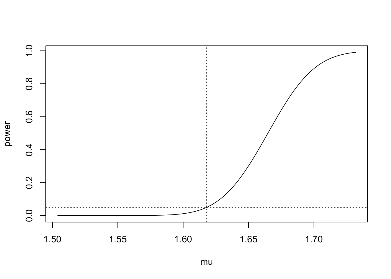
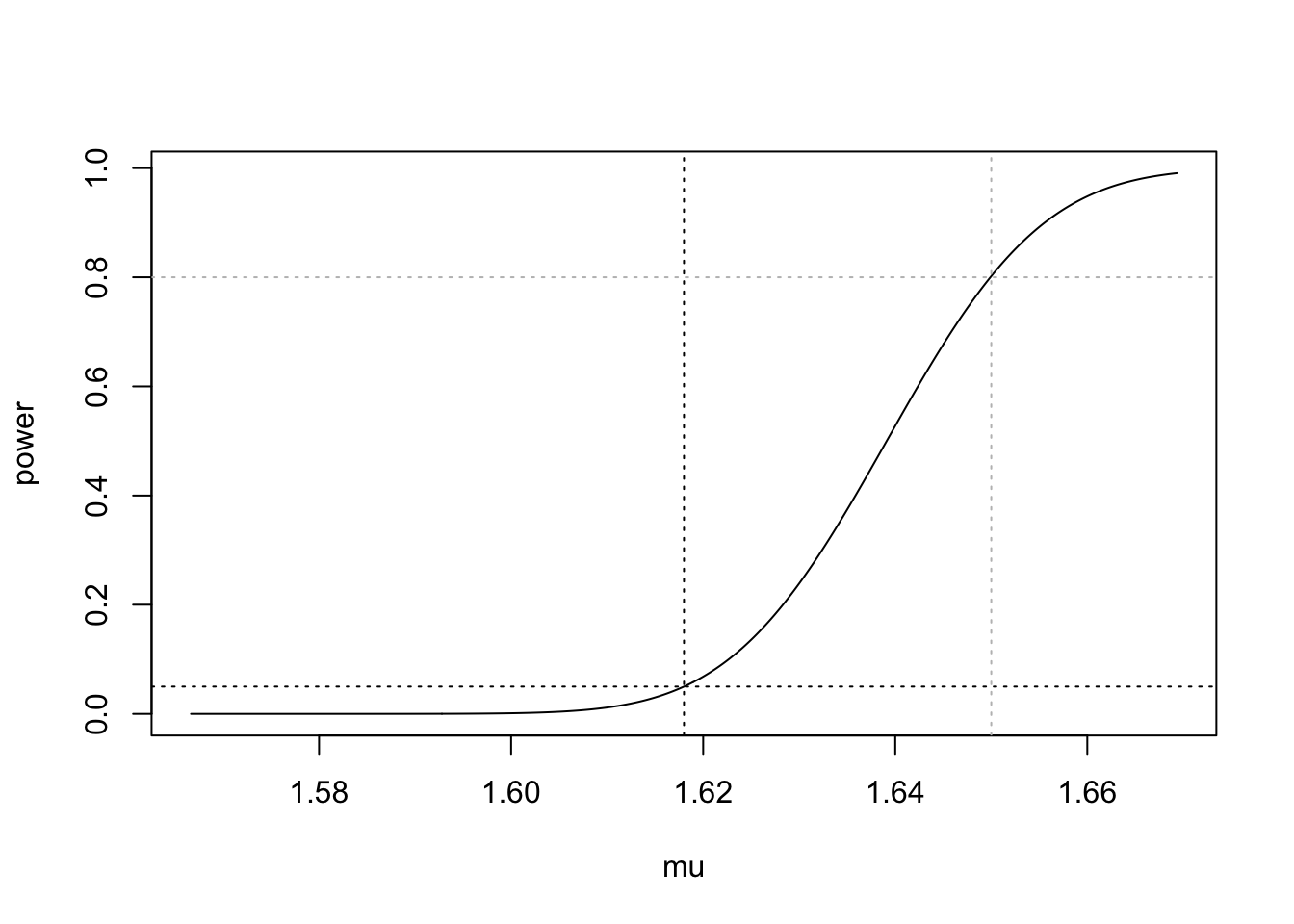
If we choose some values for \(\mu_0\), \(\sigma\), \(\alpha\), and \(n\) we can make a plot of the power function. In the golden ratio example, we have \(\mu_0 = 1.618\) and \(n = 27\), and we are free to choose any significance level we wish for carrying out the test; suppose we choose \(\alpha = 0.05\). The tricky part is that we do not know the variance \(\sigma\) in the case of the golden ratio data (indeed, in practice we will seldom, if ever, know the true value of \(\sigma\)). We will therefore use the sample standard deviation \(S_n\) as a guess for \(\sigma\). For the golden ratio data we obtain \(S_n = 0.148\). Plugging this in for \(\sigma\), we can make a plot of the power curve for the right-sided test as in Figure 37.1.
Note that when the true value of \(\mu\) is equal to the null value \(\mu_0 = 1.618\) (indicated by the vertical dotted line), the power of the test is exactly equal to the significance level \(\alpha\) (indicated by the horizontal dotted line). As the true value of \(\mu\) increases, the power, that is the probability of rejecting the null hypothesis, increases. For large enough \(\mu\), it becomes nearly a certainty that the data in a sample of size \(n = 27\) will lead to a rejection of \(H_0\). On the other hand, if the true value of \(\mu\) is less than \(\mu_0\), the probability of rejecting the null hypothesis falls below the significance level; as \(\mu\) decreases, it becomes increasingly unlikely that one would observe data leading to the rejection of \(H_0\): \(\mu \leq \mu_0\).
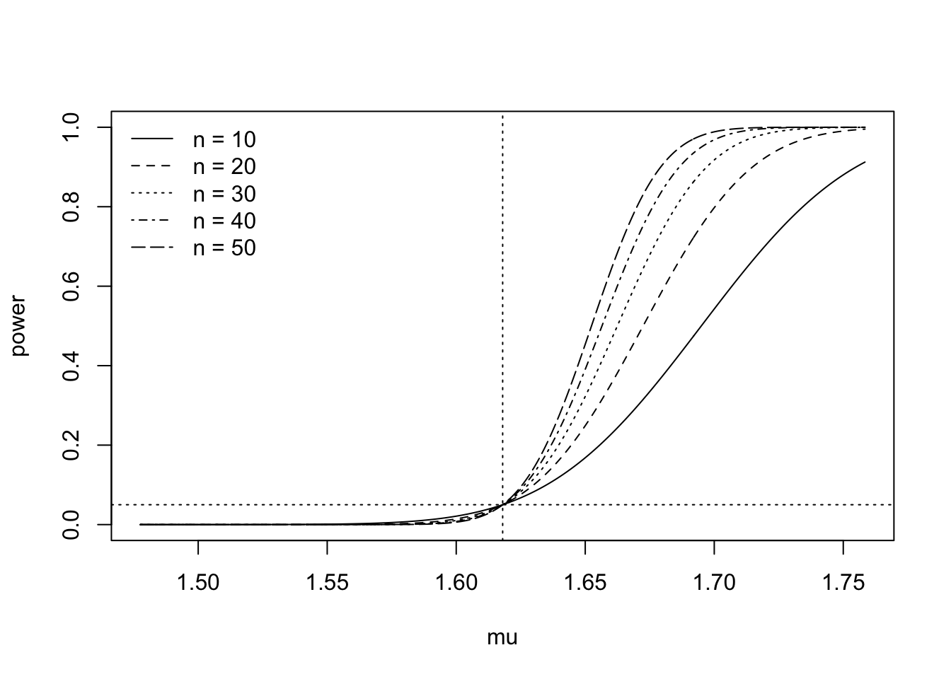
In order to understand the effect of the sample size \(n\) on the power, we can study the expression for the power and see that a larger \(n\) will increase the value of \(\gamma(\mu)\) when \(\mu > \mu_0\) and that it will decrease the value of \(\gamma(\mu)\) when \(\mu < \mu_0\). When \(\mu = \mu_0\), changing the sample size will have no effect on the power, since test is calibrated, for all sample sizes, to have size equal to \(\alpha\). Figure 37.2 shows a plot of the power curve for the golden ratio example under several sample sizes.
Figure 37.2: Power curve of right-sided test for several sample sizes
We see that for larger sample sizes, the power curve increases more quickly as a function of \(\mu\). Suppose \(\mu=1.7\). Then with a sample size of \(n = 50\), one is almost certain to reject the null hypothesis; however, if one draws a sample only of size \(n = 10\), there is only about a \(60\%\) chance the data will lead to the rejection of \(H_0\).
The power function for the left-sided test is very similar.
37.2 Left-sided test
Suppose we are testing the left-sided set of hypotheses \[
\text{$H_0$: $\mu \geq \mu_0$ versus $H_1$: $\mu < \mu_0$},
\] where we will reject \(H_0\) if \(Z_\text{test} < -z_{\alpha}\), that is, if \(\bar X_n\) lies a sufficient number of standard deviations below the null mean \(\mu_0\). Then we can write the power function as \[
\begin{align*}
\gamma(\mu) &= P_\mu( Z_\text{test} < -z_{\alpha})\\
&= P_\mu( \frac{\bar X_n - \mu_0}{\sigma / \sqrt{n}} < - z_{\alpha})\\
&= P_\mu( \frac{\bar X_n - \mu}{\sigma / \sqrt{n}} + \frac{\mu - \mu_0}{\sigma/\sqrt{n}} < -z_{\alpha})\\
&= P( Z < - z_{\alpha} - \frac{\mu - \mu_0}{\sigma/\sqrt{n}}), \quad Z \sim \mathcal{N}(0,1)\\
&= \Phi(- z_{\alpha} - \frac{\mu - \mu_0}{\sigma/\sqrt{n}}).
\end{align*}
\]
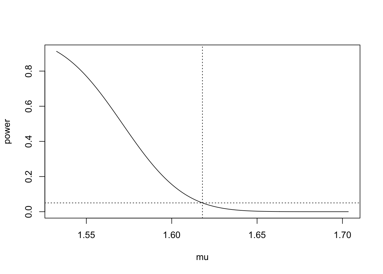
Studying this power function, we see that it is a decreasing function of \(\mu\): As \(\mu\) increases, the value inside \(\Phi(\cdot)\) decreases, so that \(\Phi(\dot)\) decreases. Plugging in \(\mu_0 = 1.618\), \(n = 27\), \(\alpha = 0.05\), and \(\sigma = 0.148\), we obtain the power curve plotted in
The power curve of the two-sided test looks quite different from those of the one-sided tests.
37.3 Two-sided test
Now suppose we are testing the two-sided set of hypotheses \[
\text{$H_0$: $\mu = \mu_0$ versus $H_1$: $\mu \neq \mu_0$},
\] where we will reject \(H_0\) if \(Z_\text{test} > |z_{\alpha/2}|\), that is, if \(\bar X_n\) lies a sufficient number of standard deviations above or below the null mean \(\mu_0\). The power function becomes \[
\begin{align*}
\gamma(\mu) &= P_\mu( Z_\text{test} > |z_{\alpha/2}|)\\
&= 1 - P_\mu( Z_\text{test} < |z_{\alpha/2}|)\\
&= 1 - P_\mu( - z_{\alpha/2} < Z_\text{test} < z_{\alpha/2})\\
&= 1 - P_\mu( - z_{\alpha/2} < \frac{\bar X_n - \mu_0}{\sigma / \sqrt{n}} < z_{\alpha/2})\\
&= 1 - P_\mu( - z_{\alpha/2} < \frac{\bar X_n - \mu}{\sigma / \sqrt{n}} +\frac{\mu - \mu_0}{\sigma/\sqrt{n}} < z_{\alpha/2})\\
&= 1 - P( - z_{\alpha/2} - \frac{\mu - \mu_0}{\sigma/\sqrt{n}} < Z < z_{\alpha/2} - \frac{\mu - \mu_0}{\sigma/\sqrt{n}}), \quad Z \sim \mathcal{N}(0,1)\\
&=1 - \Big[ \Phi(z_{\alpha/2} - \frac{\mu - \mu_0}{\sigma/\sqrt{n}}) - \Phi( - z_{\alpha/2} - \frac{\mu - \mu_0}{\sigma/\sqrt{n}})\Big]\\
&= \Phi( - z_{\alpha/2} - \frac{\mu - \mu_0}{\sigma/\sqrt{n}}) + 1 - \Phi(z_{\alpha/2} - \frac{\mu - \mu_0}{\sigma/\sqrt{n}}).
\end{align*}
\] This power function is a little more complicated, but if we look carefully, we see that it is just the sum of the two one-sided power curves with \(\alpha\) replaced with \(\alpha/2\).
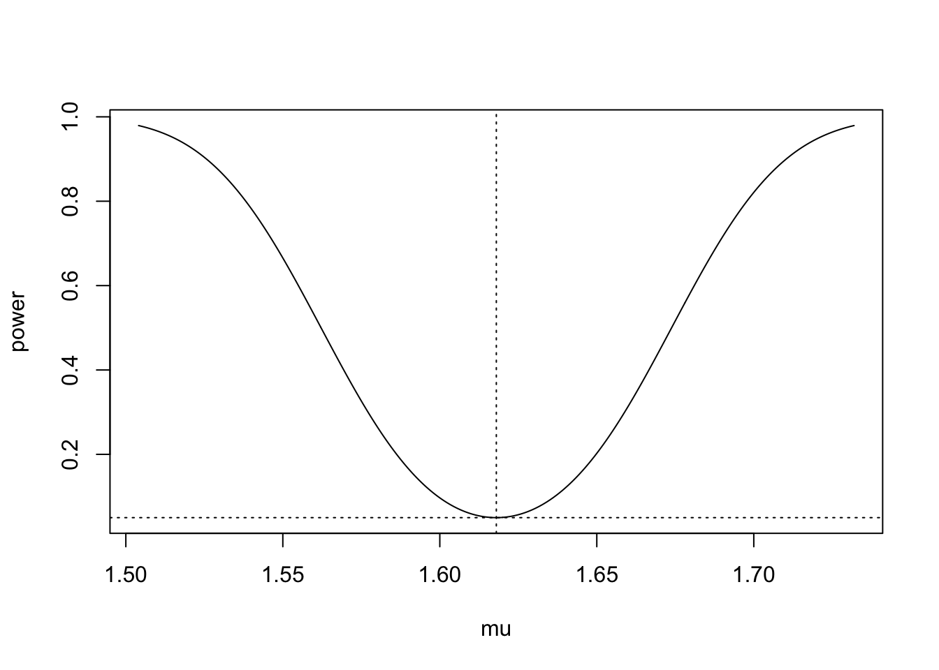
Figure 37.4 shows a plot of the power curve of the two-sided test under \(\mu_0 = 1.618\), \(n = 27\), \(\alpha = 0.05\), and \(\sigma = 0.148\).
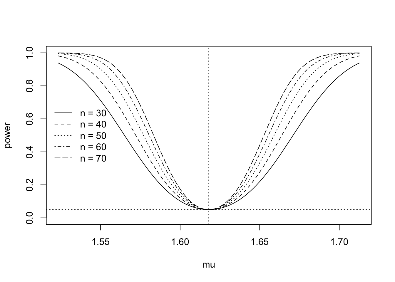
We see that in the case of the two-sided test, the probability of rejecting the null \(H_0\): \(\mu = \mu_0\) increases as \(\mu\) lies further above or below the null value \(\mu_0\). Figure 37.5 shows a plot of the power function of the two-sided test under \(\mu_0=1.618\), \(\alpha= 0.05\), and \(\sigma = 0.148\) under several sample sizes.
Figure 37.5: Power curves of two-sided test for several sample sizes
We see that larger sample sizes cause the power to increase more quickly as \(\mu\) moves from \(\mu_0\) in either direction.
37.4 Sample size based on desired power
Figure 37.2 and Figure 37.5 suggest that studying the power curve of a statistical test may help determine the size of the sample one should draw. We have seen that, given a null value \(\mu_0\) and a size \(\alpha\), one can plot the power function for many choices of the sample size \(n\), provided one has a guess for the value of the standard deviation \(\sigma\). If a guess for the value of \(\sigma\) is available, one can go about choosing a sample size as follows:
First, one must fix an alternative value \(\mu^*\) that satisfies the alternative hypothesis and is meaningfully distinct from the null value \(\mu_0\). By “meaningfully distinct” we mean that the difference between \(\mu^*\) and \(\mu\) is large enough so that the investigator would regard it as an interesting finding to conclude that \(\mu\) is equal to \(\mu^*\) instead of equal to \(\mu_0\). Having identified such a \(\mu^*\), one next specifies a desired power \(\gamma^*\). This is the smallest probability with which one wishes to reject the null hypothesis when \(\mu\) is equal to the value \(\mu^*\). With \(\mu^*\) and \(\gamma^*\) chosen, one then finds the smallest sample size \(n\) such that \(\gamma(\mu^*) \geq \gamma^*\) holds (this can be found by setting up the equation \(\gamma(\mu^*) = \gamma^*\), solving for \(n\), and rounding up to the nearest whole number.
In summary:
Fix an alternative value \(\mu^*\) and a desired power \(\gamma^*\).
Set up the equation \(\gamma(\mu^*) = \gamma^*\), solve for \(n\), and round up.
For either of the one-sided tests we discussed, we obtain the expression \[
n = \bigg\lceil \sigma^2 \Big(\frac{z_\alpha + z_{\beta^*} }{\mu^* - \mu_0}\Big)^2\bigg\rceil,
\tag{37.1}\] where \(\beta^* = 1 - \gamma^*\).
For the left-sided case, we have \[
\begin{align*}
& \gamma^* = \Phi(-z_\alpha - \frac{\mu^* - \mu_0}{\sigma / \sqrt{n}}) \\
& \iff z_{1-\gamma^*} = -z_\alpha - \frac{\mu^* - \mu_0}{\sigma / \sqrt{n}} \\
& \iff \sqrt{n} = \sigma \frac{z_\alpha-z_{\gamma^*}}{\mu^* - \mu},
\end{align*}
\] using the fact that \(z_{1-\gamma^*} = -z_{\gamma^*}\) (draw pictures to see this).
From here, note that \(z_{\gamma^*} = - z_{\beta^*}\) by the fact that \(\beta^* = 1- \gamma^*\) (draw pictures again!). This leads to Equation 37.1 in both cases.
For the two-sided test, we obtain approximately \[
n = \bigg\lceil \sigma^2 \Big(\frac{z_{\alpha/2} + z_{\beta^*} }{\mu^* - \mu_0}\Big)^2\bigg\rceil.
\tag{37.2}\]
This expression is an approximation to the value of \(n\) for which \(\gamma(\mu^*) = \gamma^*\). It is really just the one-sided calculation with \(\alpha/2\) plugged in instead of \(\alpha\). The approximation works because if \(\mu\) is to the right, say, of \(\mu_0\), chances are quite slim that you would reject \(H_0\) with a sample mean to the left of \(\mu_0\), and vice versa, so in the sample size calculation, we disregard the part of the power function corresponding to one or the other side. More precisely, in the power expression \[
\gamma(\mu) = \Phi( - z_{\alpha/2} - \frac{\mu - \mu_0}{\sigma/\sqrt{n}}) + \Big[1 - \Phi(z_{\alpha/2} - \frac{\mu - \mu_0}{\sigma/\sqrt{n}})\Big],
\] one or the other of the terms on the right hand side is assumed small enough to be negligible—the first corresponding to rejection of \(H_0\): \(\mu = \mu_0\) in favor of \(\mu < \mu_0\) and the second to rejection of the same in favor of \(\mu > \mu_0\).
Example 37.1 (Golden ratio sample size determination:) Suppose we are testing \(H_0\): \(\mu \leq 1.618\) versus \(H_1\): \(\mu > 1.618\) and that we wish to reject \(H_0\) with probability at least \(0.80\) if the true mean of the ratio \(B/A\) were equal to \(1.65\). Then using \(S_n = 0.148\) as a guess of \(\sigma\), we would use Equation 37.1 to choose the sample size.
We see that this sample size is just sufficient to give the test the desired power of \(\gamma^* = 0.80\) when the true mean is equal to \(\mu^*= 1.65\).
37.5 Power when the variance is unknown
Lastly: We have assumed throughout that \(\sigma^2\) was known. It is possible to derive the power function of the t test which one would use if \(\sigma^2\) were unknown and replaced with \(S_n^2\), leading to the test statistic \[
T_{\text{test}} = \frac{\bar X_n - \mu_0}{S_n/\sqrt{n}},
\] however, these investigations involve versions of the t distributions called non-central t-distributions, which are beyond the scope of an introductory statistics course. However, of large sample sizes it will not make much difference whether one uses the calculation derived here or exact calculations based on non-central t distributions, so the omission of the latter from our discussion is not so costly in the end.
37.6 Power for other kinds of tests
We have restricted our discussion of power to one-sample tests concerning the mean of a Normal population. However, every statistical test has a power function! The examples we covered here are merely a good starting point for understanding statistical power.