Here we return to the sampling distribution of the sample mean \(\bar X_n\). In Chapter 16 we learned if \(X_1,\dots,X_n\) is a random sample from a population with mean \(\mu\) and variance \(\sigma^2\), then the sample mean \(\bar X_n\) has mean \(\mu\) and variance \(\sigma^2/n\). Moreover, we learned that if the population distribution is a normal distribution, \(\bar X_n\) has the \(\mathcal{N}(\mu,\sigma^2/n)\) distribution. This fact was helpful to us when we wanted to compute probabilities concerning \(\bar X_n\).
It is often the case, however, that the population distribution is not a normal distribution, for which case we have not yet discussed how to compute probabilities about \(\bar X_n\) (Why is it so important for us to compute probabilities about \(\bar X_n\)? We’ll discuss this more later on, but \(\bar X_n\) is our best guess of the value of the unknown population mean \(\mu\). If we are to learn this unknown value, we would like to know where\(\bar X_n\) is likely to lie with respect to this unknown value. The sampling distribution of \(\bar X_n\) carries this information.).
When the population distribution is not normal, an important result in probability tells us that as long as the sample size \(n\) is large, \(\bar X_n\) will have a probability distribution which is approximately a normal distribution. This result is called the central limit theorem. It states that if I send \(\bar X_n\) into the “\(Z\) world,” as it were, by standardizing it as \[
Z_n = \frac{\bar X_n - \mu}{\sigma / \sqrt{n}},
\] then this \(Z_n\) will have approximately the same distribution as \(Z \sim \mathcal{N}(0,1)\) as long as \(n\) is large. We state the result somewhat informally here:
Proposition 21.1 (Central limit theorem) Let \(X_1,\dots,X_n\) be a random sample from a non-normal population with mean \(\mu\) and \(\sigma^2 < \infty\). Then \[
Z_n = \frac{\bar X_n - \mu}{\sigma / \sqrt{n}} \text{ behaves more and more like } Z \sim \mathcal{N}(0,1)
\] for larger and larger \(n\).
There is a requirement in the above proposition that the population variance \(\sigma^2\) must be less than infinity. This requirement may seem unnecessary, but there exist some probability distributions for which the variance does not exist (recall that the variance is computed as a sum or as an integral, depending on whether the random variable is discrete or continuous, and it is possible that the sum or integral will diverge to infinity). The condition \(\sigma^2 < \infty\) rules out random samples from such distributions.
Saying that a random variable “behaves more and more like” another for “larger and larger \(n\)” describes a concept in probability called convergence in distribution, the precise details of which lie beyond the scope of this text. It will suffice for us to understand the proposition as saying that if \(n\) is large enough, we can pretend that \(Z_n\) has the \(\mathcal{N}(0,1)\) distribution with only a negligible loss of accuracy in any probabilities we compute based on pretending this.
It follows from the proposition that for large enough \(n\), the sample mean \(\bar X_n\) has approximately the \(\mathcal{N}(\mu,\sigma^2/n)\) distribution. To express this we may write \[
\bar X_n \overset{\operatorname{approx}}{\sim} \mathcal{N}\Big(\mu,\frac{\sigma^2}{n}\Big)
\tag{21.1}\] for large \(n\).
How large must \(n\) be, one may wonder, before one can pretend that \(\bar X_n\) has the \(\mathcal{N}(\mu,\sigma^2/n)\) distribution? It really depends on properties of the population distribution: If the population distribution is very skewed or very heavy tailed, one may need quite a large sample size \(n\) in order for \(\bar X_n\) to behave like a normally distributed random variable. However, if the population distribution is symmetric and not heavy-tailed, \(\bar X_n\) will behave like a normally distributed random variable even when the sample size is quite small. It may also make a difference whether the random variables in random sample are discrete or continuous. For whatever reason, the rule of thumb that \(n\) should be at least \(30\) seems to have emerged as standard.
If we can assume \(\bar X_n \overset{\operatorname{approx}}{\sim} \mathcal{N}(\mu,\sigma^2/n)\), then we can proceed with computing probabilities concerning \(\bar X_n\) just as we did in Chapter 16 in the case in which the sample was drawn from the \(\mathcal{N}(\mu,\sigma^2)\) distribution.
Exercise 21.1 (Mean of die rolls) Let \(X_1,\dots,X_n\) denote \(n\) rolls of a six-sided die.
Give the expected value and variance of \(\bar X_n = n^{-1}(X_1+\dots + X_n)\).2
Give an approximation to the probability that the mean of \(50\) rolls will be less than \(3\).3
Give an approximation to the probability that the sum of 50 rolls will be at least \(180\).4
Give an approximation to \(P(|\bar X_n - 7/2| > 1/4)\) when \(n = 50\).5
Code
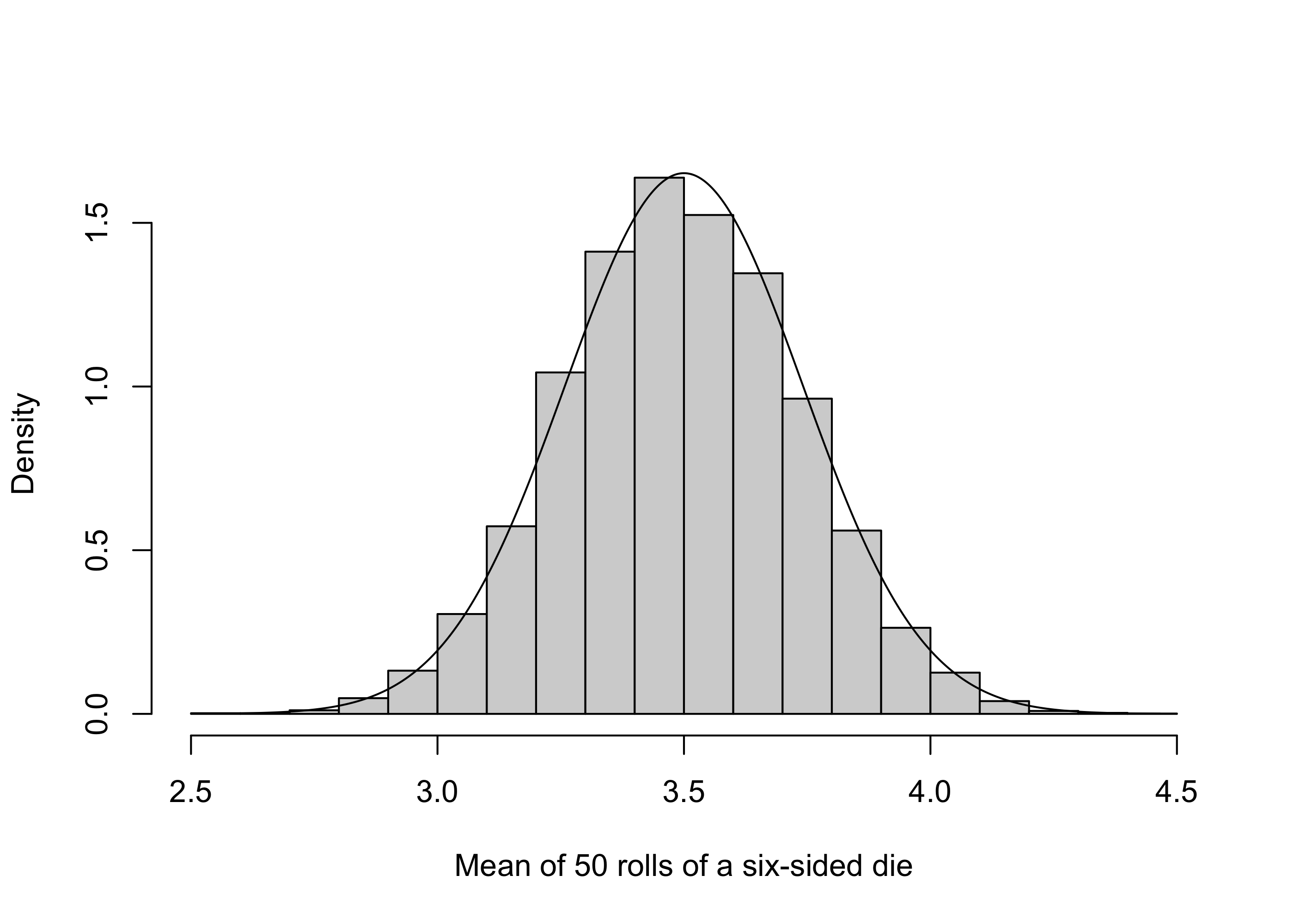
n <-50S <-1e4X <-matrix(sample(1:6,n*S,replace=T),S,n)Xbar <-apply(X,1,mean)hist_Xbar <-hist(Xbar,breaks=20,plot=F)sg <-sqrt((35/12)/n)mu <-7/2x <-seq(mu -4*sg,mu+4*sg,length=501)fx <-dnorm(x,mu,sg)par(bg =NA)plot(hist_Xbar,main ='',freq = F,ylim =c(0,max(hist_Xbar$density,fx)),xlab ='Mean of 50 rolls of a six-sided die')lines(fx~x)
Figure 21.1: Histogram of \(10^5\) realizations of the mean of \(50\) rolls of a six-sided die with PDF of the \(\mathcal{N}(7/2,(35/12)/50)\) distribution overlaid.
Example 8.4 gives \(\mathbb{E}X_1 = 7/2\) and Exercise 8.3 gives \(\operatorname{Var}X_1= 35/12\). It is the same for any of the random variables in the sample since they are identically distributed.↩︎
We have \(\mathbb{E}\bar X_n = 7/2\) and \(\operatorname{Var}\bar X_n = (35/12) / n\).↩︎
Since \(n=50\) is large, \(\bar X_n\) follows approximately the \(\mathcal{N}(7/2,(35/12)/50)\) distribution. So \[
\begin{align*}
P(\bar X_n < 3) &= P\Big(\frac{\bar X_n - 7/2}{\sqrt{(35/12)/50}} < \frac{3 - 7/2}{\sqrt{(35/12)/50}}\Big) \\
&\approx P(Z < -2.0702)\\
&=0.0192.
\end{align*}
\]↩︎
Note that the sum \(X_1+\dots + X_n\) is equal to \(n \bar X_n\). So we may write \[
\begin{align*}
P(50 \bar X_n \geq 180 ) &= P(\bar X_n \geq 180/50 )\\
&=P\Big(\frac{\bar X_n - 7/2}{\sqrt{(35/12)/50}} < \frac{180/50 - 7/2}{\sqrt{(35/12)/50}}\Big) \\
&\approx P(Z > 0.4140)\\
&=0.3394.
\end{align*}
\]↩︎