We now understand how to test hypotheses about the mean \(\mu\) when this is the mean of a normal population from which we have drawn a random sample. If the population standard deviation \(\sigma\) is known, we compute \(Z_{\operatorname{test}}\) as in Equation 32.1, and compare the value of this test statistic to a critical value as in Proposition 32.1; if \(\sigma\) is unknown, we replace it with the sample standard deviation \(S_n\) and compute \(T_{\operatorname{test}}\) as in Equation 33.1, and compare its value to a critical value as in Proposition 33.1.
However, we have not yet discussed how to test hypotheses about a mean \(\mu\) when this is not the mean of a normally distributed population but of a population with some non-normal distribution. As in the case of constructing confidence intervals, the Central Limit Theorem in Proposition 21.1 allows us to base inferences on the assumption that the sample mean is approximately normally distributed when the sample size is large.
Suppose \(X_1,\dots,X_n\) is a random sample from some distribution with mean \(\mu\) and variance \(\sigma^2\), and, letting \(\mu_0\) denote some null value for \(\mu\), consider testing one of the sets of hypotheses:
\(H_0\): \(\mu \leq \mu_0\) versus \(H_1\): \(\mu > \mu_0\)
\(H_0\): \(\mu \geq \mu_0\) versus \(H_1\): \(\mu < \mu_0\)
\(H_0\): \(\mu = \mu_0\) versus \(H_1\): \(\mu \neq \mu_0\)
We will ignore the \(\sigma\)-known case, as one rarely encounters it in practice, and assume that \(\sigma\) needs to be estimated. Since \(S_n\) is an estimator which can be counted on to take values closer and closer to \(\sigma\) for larger and larger \(n\), we have \[
\frac{\bar X_n - \mu}{S_n /\sqrt{n}} \overset{\operatorname{approx}}{\sim}\mathcal{N}(0,1),
\] for large enough \(n\), as stated in Proposition 28.1. In consequence, even when the population distribution is not a normal distribution, one can test the above sets of hypotheses as described here:
Proposition 34.1 (Large-sample tests of hypotheses for a mean) Let \(X_1,\dots,X_n\) be a random sample from a distribution with mean \(\mu\) and variance \(\sigma^2 < \infty\). Then the following tests have size closer and closer to \(\alpha\) for larger and larger \(n\):
For \(H_0\): \(\mu \leq \mu_0\) versus \(H_1\): \(\mu > \mu_0\), reject \(H_0\) if \(T_{\operatorname{test}}> z_\alpha\).
For \(H_0\): \(\mu \geq \mu_0\) versus \(H_1\): \(\mu < \mu_0\), reject \(H_0\) if \(T_{\operatorname{test}}< -z_\alpha\).
For \(H_0\): \(\mu = \mu_0\) versus \(H_1\): \(\mu \neq \mu_0\), reject \(H_0\) if \(|T_{\operatorname{test}}| > z_{\alpha/2}\).
Note that one could replace \(z_{\alpha}\) and \(z_{\alpha/2}\) in the above with \(t_{n-1,\alpha}\) and \(t_{n-1,\alpha/2}\), which would make the rejection rules above coincide exactly with those prescribed in Proposition 33.1, and the statement of the proposition would be equally true, because as \(n\) increases, the \(t_{n-1}\) distribution becomes more and more like the \(\mathcal{N}(0,1)\) distribution. For \(n \geq 30\), however, it does not make much of a difference; for example, with \(n = 30\) and \(\alpha = 0.05\), we have \(t_{30-1,0.05} = 1.699127\), while \(z_{0.05} = 1.6448536\), and \(t_{30-1,0.025} = 2.0452296\), while \(z_{0.025} = 1.959964\). One can look at the last few rows of the \(t\) table in Chapter 46 to compare more upper quantiles of the standard normal and \(t\) distributions. The reason we have preferred to use the critical values \(z_\alpha\) and \(z_{\alpha/2}\) in the large-sample case, even when \(\sigma\) is unknown, is that the \(t\) distribution only truly arises when one’s random sample is drawn from a normal distribution. If the sample is not drawn from a normal distribution, then it is somewhat arbitrary to use \(t\) distribution quantiles as critical values.
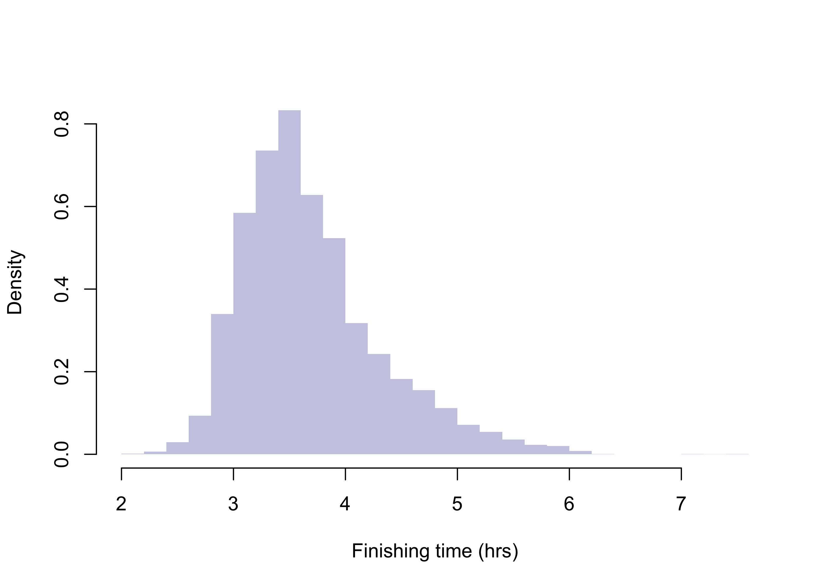
Exercise 34.1 (2009 Boston Marathon mens finishing times) Refer to the data in Example 17.1 and regard the mens finishing times as a population of values
The population has mean \(\mu = 3.693\) and standard deviation \(\sigma = 0.628\), but suppose we don’t know these values, and we draw a random sample of size \(n = 50\), obtaining \(\bar X_n = 3.667\) and \(S_n = 0.582\). Test the following sets of hypotheses at significance level \(\alpha = 0.01\), stating whether your conclusion is a Type I error, a Type II error, or a correct decision:
\(H_0\): \(\mu \leq 3.75\) versus \(H_1\): \(\mu > 3.75\).1
\(H_0\): \(\mu \geq 3.75\) versus \(H_1\): \(\mu < 3.75\). 2
\(H_0\): \(\mu = 3.75\) versus \(H_1\): \(\mu \neq 3.75\).3
Figure 34.1 summarizes when to use which test statistic, \(Z_{\operatorname{test}}\) or \(T_{\operatorname{test}}\), and to which critical value, \(z_{\alpha}\) or \(t_{n-1,\alpha}\), to compare it when testing \(H_0\): \(\mu \leq \mu_0\) versus \(H_0\): \(\mu > \mu_0\). Appropriate rejection rules when testing the left-sided and two-sided sets of hypotheses are similarly summarized.
---
config:
  look: handDrawn
---
flowchart LR
  %% root
  Root["Population distribution"]

  %% bags
  normal["$$\sigma^2$$"]
  nonnormal["$$n$$"]

  %% root -> bags (edge labels)
  Root -->|normal|normal
  Root -->|not normal|nonnormal

  %% normal leaves
  normal_known["$$Z_{\text{test}} > z_\alpha$$"]
  normal_unknown["$$T_{\text{test}} > t_{n-1,\alpha}$$"]
  normal -->|known| normal_known
  normal -->|unknown| normal_unknown

  %% nonnormal leaves
  nonnormal_geq30["$$\sigma^2$$"]

  nonnormal --> |at least 30|nonnormal_geq30
  nonnormal --> |less than 30|nonnormal_lt30

  nonnormal_geq30_known["$$Z_{\text{test}} > z_\alpha$$"]
  nonnormal_geq30_unknown["$$T_{\text{test}} > z_{\alpha}$$"]

  nonnormal_lt30["Can do nothing so far"]

  nonnormal_geq30 -->|known| nonnormal_geq30_known
  nonnormal_geq30 -->|unknown| nonnormal_geq30_unknown
Figure 34.1: Rejection rules for testing the right-sided set of hypotheses about a mean.
The null hypothesis is true, so a correct decision is not to reject it. We begin by computing the test statistic \[
T_{\operatorname{test}}= \frac{3.667 - 3.75}{0.582/\sqrt{50}} = -1.008.
\] The sample mean \(\bar X_n < 3.75\) carries evidence in favor of \(H_0\), so we have no grounds to reject it. This is reflected in the negative value of the test statistic. ↩︎
The null hypothesis is false, so the correct decision is to reject it. We will reject \(H_0\) if the test statistic lies below the critical value \(-z_{0.01} = -2.326\). This is not the case, so we fail to reject \(H_0\), making a Type II error.↩︎
Again, the null hypothesis is false, so the correct decision is to reject it. We will reject \(H_0\) if the test statistic exceeds in magnitude the critical value \(z_{0.01/2} = 2.576\). This is not the case, so we fail to reject \(H_0\), again making a Type II error.↩︎