Until now we have considered what we can learn from a random sample about the mean or variance or proportion of “successes” in the population from which the sample was drawn. It is often of interest to learn not only about a single population, but about two separate populations by drawing a random sample from each one. In particular, it is often of interest to compare the means of the two populations (or the variances, or the proportions of “successes”). Here we will consider how to learn from random samples drawn independently from separate populations about the difference between the means of the populations.
To set up our notation, we will suppose that we draw a random sample of size \(n_1\) from the first population, denoting the values in this sample by \(X_{11},\dots, X_{1n_1}\) and that we draw \(n_2\) values from the second population, denoting the values in this random sample as \(X_{21},\dots,X_{2n_2}\). This way \(X_{ij}\) represents value \(j\) drawn from population \(i\) for \(i=1,2\), where the index \(j\) takes the values \(j = 1,\dots,n_i\). Moreover, we will compute on each sample \(i=1,2\) the sample mean \[
\bar X_i = \frac{1}{n_i}\sum_{j=1}^{n_i} X_{ij},
\] so that \(\bar X_1\) and \(\bar X_2\) denote the two sample means, and the sample variance \[
S_i^2 = \frac{1}{n_i - 1}\sum_{j=1}^{n_i}(X_{ij} - \bar X_i)^2,
\] so that \(S_1\) and \(S_2\) denote the two sample standard deviations.
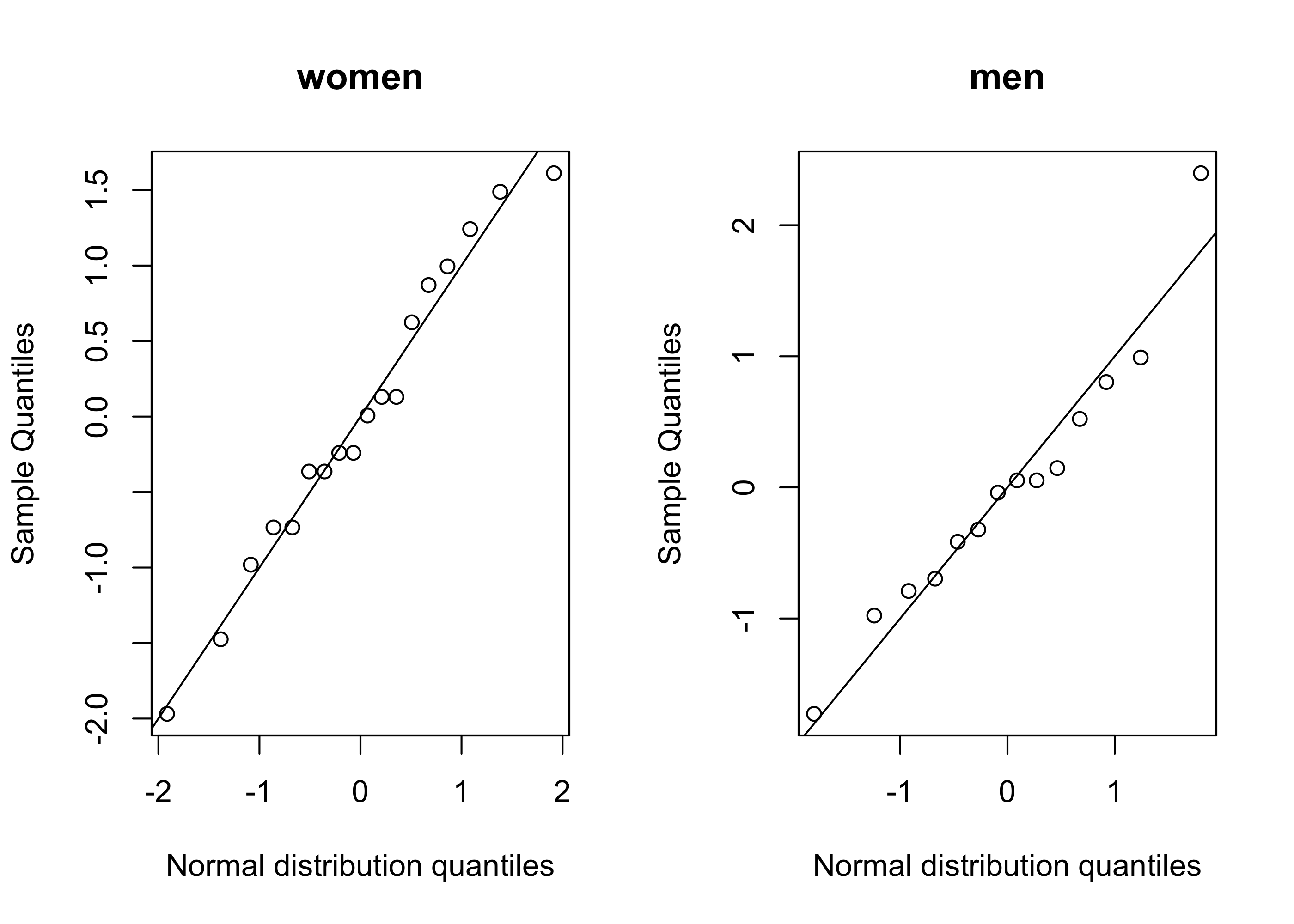
At first we will assume that each sample has been drawn from a normal distribution. That is, we will assume \[
X_{i1},\dots,X_{in_i} \overset{\text{ind}}{\sim}\mathcal{N}(\mu_i,\sigma_i^2)
\] for \(i = 1,2\), so that \(\mu_1\) and \(\mu_2\) are the two population means and \(\sigma_1^2\) and \(\sigma_2^2\) are the two population variances. Here is an example of a study involving two random samples:
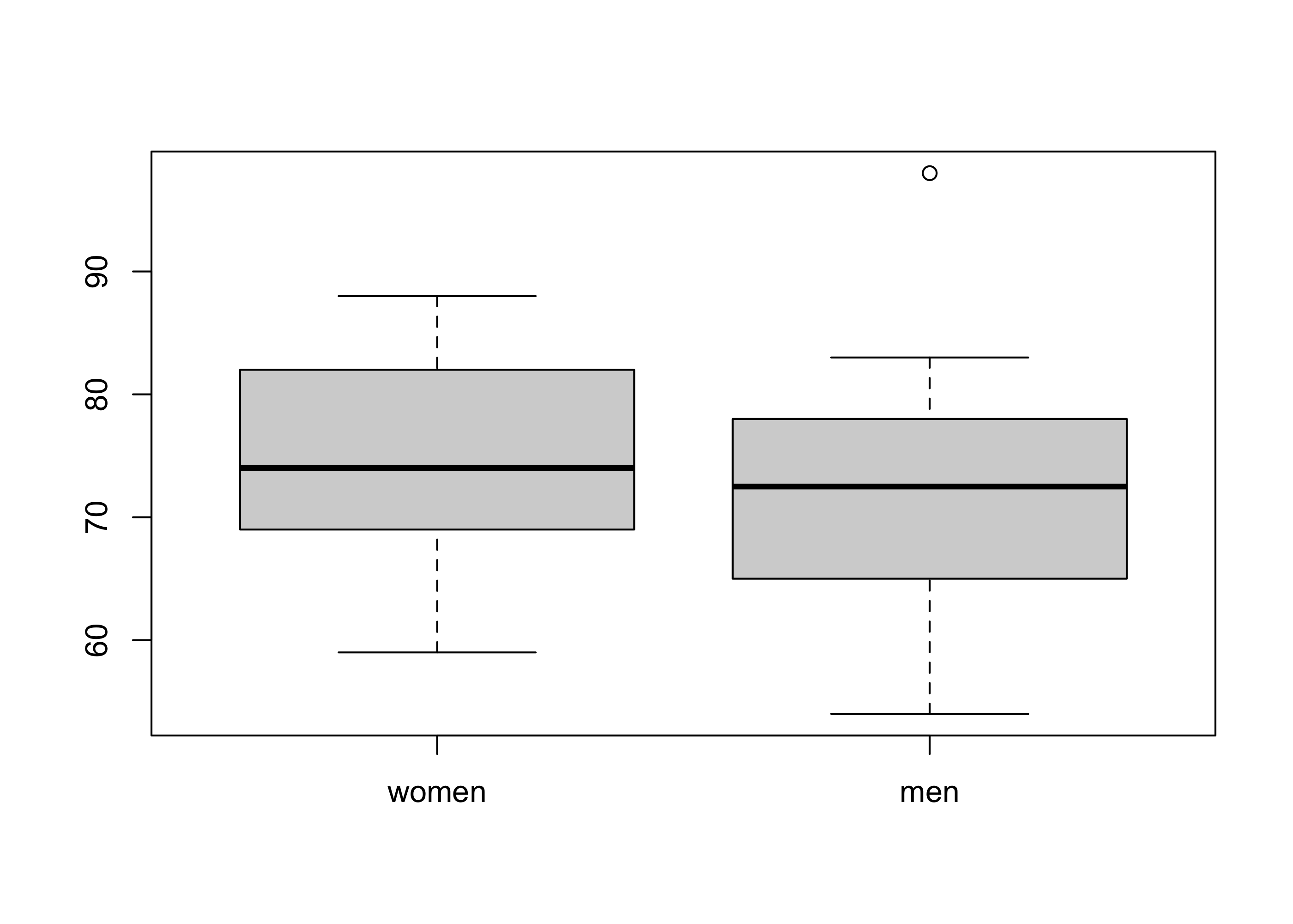
Example 38.1 (Resting heart rates of men and women) In a class with \(14\) male students and \(18\) female students, each student was asked to measure his or her heart rate. During two 30-second periods separated by several minutes, students were asked to count the number of heartbeats they felt. These counts were added to obtain for each student a heart rate measurement in beats per minute (bpm). It is reported that women have, on average, a higher resting heart rate than men. Does this show up in the data collected here?
par(mfrow=c(1,2),bg =NA)qqnorm(scale(hr_w),main ="women",xlab ="Normal distribution quantiles")abline(0,1)qqnorm(scale(hr_m),main ="men",xlab ="Normal distribution quantiles")abline(0,1)
In the resting heart rates example, we could let \(\mu_1\) represent the mean resting heart rate for women and \(\mu_2\) that of men (it does not matter which group is considered group 1). Then we are interested in learning whether \(\mu_1 > \mu_2\), as is reported. If we are interested in making comparisons between two population means, as we are in this case, it is often sensible to regard the difference \(\mu_1 - \mu_2\) as the object of estimation and inference. That is, we can answer questions about how \(\mu_1\) and \(\mu_2\) compare to each other by constructing confidence intervals for or testing hypotheses concerning the difference \(\mu_1 - \mu_2\).
We first consider how to construct confidence intervals for the difference \(\mu_1 - \mu_2\).
38.1 Confidence intervals for a difference in means
Our first step will be to consider the behavior of our best guess of the difference \(\mu_1 - \mu_2\) based on the data: this is the difference \(\bar X_1 - \bar X_2\). We will use the following result as a starting point:
Proposition 38.1 (Distribution of a difference in sample means) If \(X_{i1},\dots,X_{in_i} \overset{\text{ind}}{\sim}\mathcal{N}(\mu_i,\sigma_i^2)\) for \(i=1,2\) are independent random samples then \[
\bar X_1 - \bar X_2 \sim \mathcal{N}\Big(\mu_1 - \mu_2,\frac{\sigma^2_1}{n_1} + \frac{\sigma_2^2}{n_2}\Big),
\] so that \[
\frac{\bar X_1 - \bar X_2 - (\mu_1 - \mu_2)}{\sqrt{\dfrac{\sigma^2_1}{n_1} + \dfrac{\sigma_2^2}{n_2}}} \sim \mathcal{N}(0,1).
\]
The above result tells us how we can send the difference in sample means \(\bar X_1 - \bar X_2\) into the \(Z\) world, or the number-of-standard-deviations world, so that the result is a standard normal random variable. If the population variances \(\sigma_1^2\) and \(\sigma_2^2\) were known to us, then we could use the above result to construct confidence intervals for or test hypotheses about the difference \(\mu_1 - \mu_2\) based on the value of \(\bar X_1 - \bar X_2\) obtained from our sample data. However, it is seldom (basically never) the case in practice that we know the values of \(\sigma_1^2\) and \(\sigma_2^2\); we must estimate them from the sample data.
The most natural way to estimate the population variances \(\sigma_1^2\) and \(\sigma_2^2\) is with the corresponding sample variances \(S_1^2\) and \(S_2^2\). Previously, whenever we replaced an unknown population standard deviation with its sample counterpart, a \(t\) distribution arose. This will also be the case in the two-sample setup we are considering at present, but with an extra complication: If we replace \(\sigma_1^2\) and \(\sigma_2^2\) by \(S_1^2\) and \(S_2^2\), respectively, we find that the Studentized quantity \[
\frac{\bar X_1 - \bar X_2 - (\mu_1 - \mu_2)}{\sqrt{\dfrac{S^2_1}{n_1} + \dfrac{S^2_2}{n_2}}}
\] does not have exactly a \(t\) distribution, but rather a distribution which to which a \(t\) distribution with carefully chosen degrees of freedom can serve as a good approximation. We state the result:
Proposition 38.2 (Studentized difference in means with Satterthwaite) If \(X_{i1},\dots,X_{in_i} \overset{\text{ind}}{\sim}\mathcal{N}(\mu_i,\sigma_i^2)\) for \(i=1,2\) are independent random samples then \[
\frac{\bar X_1 - \bar X_2 - (\mu_1 - \mu_2)}{\sqrt{\dfrac{S^2_1}{n_1} + \dfrac{S^2_2}{n_2}}} \overset{\operatorname{approx}}{\sim}t_{\nu},
\] where \(\nu\) is the degrees of freedom value given by \[
\nu = \Big(\frac{S_1^2}{n_1} + \frac{S_2^2}{n_2} \Big)^2\Big[ \frac{(S_1^2/n_1)^2}{n_1-1} + \frac{(S_2^2/n_2)^2}{n_2-1}\Big]^{-1}.
\tag{38.1}\]
The use of the \(t\) distribution with degrees of freedom chosen as above to approximate the distribution of Studentized difference in sample means is called the Satterthwaite or the Welch or the Welch-Satterthwaite approximation. In consequence of the above result, we can define an approximate \((1-\alpha)100\%\) confidence interval for \(\mu_1 - \mu_2\) as stated next:
Proposition 38.3 (Satterthwaite confidence interval for difference in means) If \(X_{i1},\dots,X_{in_i} \overset{\text{ind}}{\sim}\mathcal{N}(\mu_i,\sigma_i^2)\) for \(i=1,2\) are independent random samples then the interval with endpoints \[
\bar X_1 - \bar X_2 \pm t_{\nu,\alpha/2} \sqrt{\frac{S_1^2}{n_1} + \frac{S_2^2}{n_2}}
\] will contain the difference \(\mu_1 - \mu_2\) with probability approximately \(1-\alpha\), where \(\nu\) is given in Equation 38.1.
In the next exercise the above interval is computed to compare the mean resting heart rates of men and women based on the data in Example 38.1.
Exercise 38.1 (Resting heart rates continued) For the resting heart rate data of Example 38.1 we obtain, treating women as population \(1\), \(\bar X_1 = 74.944\), \(\bar X_2 = 72.429\), \(S_1 = 8.098\), and \(S_2 = 10.668\), with \(n_1 = 18\) and \(n_2 = 14\). Construct a confidence interval for \(\mu_1 - \mu_2\) at levels:
It it somewhat of a nuisance to compute the degrees of freedom given in Equation 38.1. It turns out one can Studentize the difference \(\bar X_1 - \bar X_2\), that is, one can send this into the \(T\) world—the number-of-estimated-standard-deviations world—more elegantly if one is willing to make the assumption that the variances \(\sigma_1^2\) and \(\sigma_2^2\) of the two population are equal to each other. In particular, if \(\sigma_1^2 = \sigma_2^2 = \sigma^2\) for some \(\sigma^2\), one can estimate the common variance \(\sigma^2\) with \[
\hat \sigma^2 = \frac{(n_1-1)S_1^2 + (n_2 - 1)S_2^2}{n_1 + n_2 - 2},
\tag{38.2}\] which pools the values in both samples together in the estimation of \(\sigma^2\). Then we have the following result:
Proposition 38.4 (Studentized difference in means) If \(X_{i1},\dots,X_{in_i} \overset{\text{ind}}{\sim}\mathcal{N}(\mu_i,\sigma^2)\) for \(i=1,2\) are independent random samples then \[
\frac{\bar X_1 - \bar X_2 - (\mu_1 - \mu_2)}{\hat \sigma \sqrt{\dfrac{1}{n_1} + \dfrac{1}{n_2}}} \sim t_{n_1 + n_2 - 2}.
\]
In consequence of the above, we may, if the two populations have common variance \(\sigma^2\), construct a confidence interval for the difference \(\mu_1 - \mu_2\) as in the next result:
Proposition 38.5 (Pooled variance confidence interval for difference in means) If \(X_{i1},\dots,X_{in_i} \overset{\text{ind}}{\sim}\mathcal{N}(\mu_i,\sigma^2)\) for \(i=1,2\) are independent random samples then the interval with endpoints \[
\bar X_1 - \bar X_2 \pm t_{n_1 + n_2 - 2,\alpha/2} \hat \sigma \sqrt{\frac{1}{n_1} + \frac{1}{n_2}}
\] will contain the difference \(\mu_1 - \mu_2\) with probability \(1-\alpha\), where \(\hat \sigma\) is the pooled estimate of the common standard deviation \(\sigma\) according to Equation 38.2.
The interval based on a pooled estimate of the variance is only valid if we truly have \(\sigma_1^2 = \sigma_2^2\), whereas the more complicated Satterthwaite interval is valid in either case—when the variances are equal and they are not. Thus, it may be safer to simply use the Satterthwaite method by default.
Exercise 38.2 (Resting heart rates with pooled variance) Based on the data in Example 38.1, treating women as population 1, construct the pooled variance confidence interval for \(\mu_1 - \mu_2\) at levels:
If the sample sizes \(n_1\) and \(n_2\) are both large, the following result justifies the construction of a confidence interval for \(\mu_1-\mu_2\) without using the \(t\)-distribution:
Proposition 38.6 (Large-sample distribution of studentized difference in means) If \(X_{i1},\dots,X_{in_i}\) for \(i=1,2\) are independent random samples from distributions with means \(\mu_1\) and \(\mu_2\) and variances \(\sigma_1^2 <\infty\) and \(\sigma_2^2< \infty\), then \[
\frac{\bar X_1 - \bar X_2 - (\mu_1 - \mu_2)}{\sqrt{\dfrac{S^2_1}{n_1} + \dfrac{S^2_2}{n_2}}} \text{ behaves more and more like } Z \sim \mathcal{N}(0,1)
\] for larger and larger \(n_1\) and \(n_2\).
The above result implies:
Proposition 38.7 (Large-sample confidence interval for difference in means) If \(X_{i1},\dots,X_{in_i}\) for \(i=1,2\) are independent random samples from distributions with means \(\mu_1\) and \(\mu_2\) and variances \(\sigma_1^2 <\infty\) and \(\sigma_2^2< \infty\), then the interval with endpoints \[
\bar X_1 - \bar X_2 \pm z_{\alpha/2}\sqrt{\frac{S_1^2}{n_1} + \frac{S_2^2}{n_2}}
\] contains \(\mu_1 - \mu_2\) with probability closer and closer to \(1-\alpha\) for larger and larger \(n_1\) and \(n_2\).
A rule of thumb is to require \[
\min\{n_1,n_2\} \geq 30
\tag{38.3}\] in order to use the above interval. That is, one should require that both sample sizes are at least \(30\). Given this rule of thumb, it would not be appropriate to use the large-sample interval to construct a confidence interval for the difference in mean heart rates between men and women based on the data in Example 38.1.
Below is a flowchart summarizing when to compute which of the confidence intervals presented in this section.
---
config:
  look: handDrawn
---
flowchart LR
  %% root
  Root["Population distributions"]

  %% bags
  normal["$$\sigma_1^2, \sigma_2^2$$"]
  nonnormal["$$n_1,n_2$$"]

  %% root -> bags (edge labels)
  Root -->|normal|normal
  Root -->|not normal|nonnormal

  %% normal leaves
  normal_varequal["$$\bar X_1 - \bar X_2 \pm t_{n_1 + n_2 - 2,\alpha/2}\hat \sigma \sqrt{1/n_1 + 1/n_2}$$"]
  normal_varunequal["$$\bar X_1 - \bar X_2 \pm t_{\nu,\alpha/2} \sqrt{S_1^2/n_1 + S_2^2/n_2}$$"]
  normal -->|equal| normal_varequal
  normal -->|unequal| normal_varunequal

  %% nonnormal leaves
  nonnormal_largen["$$\bar X_1 - \bar X_2 \pm z_{\alpha/2} \sqrt{S_1^2/n_1 + S_2^2/n_2}$$"]
  nonnormal_smalln["Can do nothing so far"]

  nonnormal --> |both at least 30|nonnormal_largen
  nonnormal --> |either less than 30|nonnormal_smalln
Figure 38.1: When to build which confidence interval for a difference in means.
Next we consider how to formulate and test hypotheses concerning a difference in means \(\mu_1 - \mu_2\).
38.2 Testing hypotheses about a difference in means
Here we will consider how to test hypotheses of the following forms:
In the above, the value \(\delta_0\) stands in for any null value we wish. In the case of comparing the means of two populations, \(\delta_0\) is very often chosen to be \(\delta_0 = 0\). In this case, the right-sided set of hypotheses, for example, become \(H_0\): \(\mu_1 - \mu_2 \leq 0\) versus \(H_1\): \(\mu_1 - \mu_2 > 0\), so that one tests whether \(\mu_1\) is greater than \(\mu_2\) or not. One can choose \(\delta_0 > 0\) if one wishes to test whether \(\mu_1\) exceeds \(\mu_2\) by more than some specific amount.
The result below is an immediate consequence of Proposition 38.2. It describes size-\(\alpha\) tests of hypotheses in any of the above forms when the two populations have normal distributions (regardless of whether they have equal variances):
Proposition 38.8 (Tests of hypotheses for a difference in means) Let \(X_{i1},\dots,X_{in_i} \overset{\text{ind}}{\sim}\mathcal{N}(\mu_i,\sigma_i^2)\) for \(i=1,2\) be independent random samples. Then, with \[
T_{\operatorname{test}}= \frac{\bar X_1 - \bar X_2 - \delta_0}{\sqrt{\dfrac{S_1^2}{n_1} + \dfrac{S_2^2}{n_2}}},
\] and \(\nu\) as in Equation 38.1, the following tests have size \(\alpha\):
For \(H_0\): \(\mu_1 - \mu_2 \leq \delta_0\) versus \(H_1\): \(\mu_1 - \mu_2 > \delta_0\), reject \(H_0\) if \(T_{\operatorname{test}}> t_{\nu,\alpha}\).
For \(H_0\): \(\mu_1 - \mu_2 \geq \delta_0\) versus \(H_1\): \(\mu_1 - \mu_2 < \delta_0\), reject \(H_0\) if \(T_{\operatorname{test}}< -t_{\nu,\alpha}\).
For \(H_0\): \(\mu_1 - \mu_2 = \delta_0\) versus \(H_1\): \(\mu_1 - \mu_2 \neq \delta_0\), reject \(H_0\) if \(|T_{\operatorname{test}}| > t_{\nu,\alpha/2}\).
One can obtain \(p\) values associated with the test statistic for testing any of these sets of hypotheses in the usual way—as the significance level \(\alpha^*\) which sets the critical value equal to the observed value of the test statistic (see Chapter 36).
Exercise 38.3 (Resting heart rates continued) Use the data in Example 38.1 to test, without assuming equal variances, whether the mean resting heart rate of women exceeds that of men:
By comparing the test statistic to the \(\alpha = 0.05\) critical value.5
By computing the \(p\) value and comparing it to \(\alpha = 0.05\).6
If we can assume the two populations have a common variance, Proposition 38.4 leads to the test described in the next result:
Proposition 38.9 (Tests of hypotheses for a difference in means in equal variances case) Let \(X_{i1},\dots,X_{in_i} \overset{\text{ind}}{\sim}\mathcal{N}(\mu_i,\sigma^2)\) for \(i=1,2\) be independent random samples, where \(\sigma^2\) is a common variance. Then, with \[
T_{\operatorname{test}}= \frac{\bar X_1 - \bar X_2 - \delta_0}{\hat \sigma\sqrt{\dfrac{1}{n_1} + \dfrac{1}{n_2}}},
\] and \(\hat \sigma\) as in Equation 38.2, the following tests have size \(\alpha\):
For \(H_0\): \(\mu_1 - \mu_2 \leq \delta_0\) versus \(H_1\): \(\mu_1 - \mu_2 > \delta_0\), reject \(H_0\) if \(T_{\operatorname{test}}> t_{n_1 + n_2 - 2,\alpha}\).
For \(H_0\): \(\mu_1 - \mu_2 \geq \delta_0\) versus \(H_1\): \(\mu_1 - \mu_2 < \delta_0\), reject \(H_0\) if \(T_{\operatorname{test}}< -t_{n_1 + n_2 - 2,\alpha}\).
For \(H_0\): \(\mu_1 - \mu_2 = \delta_0\) versus \(H_1\): \(\mu_1 - \mu_2 \neq \delta_0\), reject \(H_0\) if \(|T_{\operatorname{test}}| > t_{n_1 + n_2 - 2,\alpha/2}\).
As with building confidence intervals for the difference \(\mu_1 - \mu_2\), we may always use the test based on the Satterthwaite approximation, but we may only used the test which uses the pooled variance estimate when the variances of the two populations can be assumed equal. The reason for looking at the side-by-side boxplots in Example 38.1 is to ascertain whether it is plausible that the variances of the two populations might be equal.
Exercise 38.4 (Resting heart rates continued) Use the data in Example 38.1 to test, while assuming the two populations have equal variances, whether the mean resting heart rate of women exceeds that of men:
By comparing the test statistic to the \(\alpha = 0.05\) critical value.7
By computing the \(p\) value and comparing it to \(\alpha = 0.05\).8
Lastly, if the sample sizes \(n_1\) and \(n_2\) are both large, one can use the central limit result in Proposition 38.6 to justify the following large-sample tests:
Proposition 38.10 (Tests of hypotheses for a difference in means in equal variances case) Let \(X_{i1},\dots,X_{in_i}\) for \(i=1,2\) be independent random samples from distributions with means \(\mu_1\) and \(\mu_2\) and variances \(\sigma_1^2 <\infty\) and \(\sigma_2^2< \infty\). Then, with \[
T_{\operatorname{test}}= \frac{\bar X_1 - \bar X_2 - \delta_0}{\sqrt{\dfrac{S_1^2}{n_1} + \dfrac{S_2^2}{n_2}}},
\] the following tests have size closer and closer to \(\alpha\) for larger and larger \(n_1\) and \(n_2\):
For \(H_0\): \(\mu_1 - \mu_2 \leq \delta_0\) versus \(H_1\): \(\mu_1 - \mu_2 > \delta_0\), reject \(H_0\) if \(T_{\operatorname{test}}> z_\alpha\).
For \(H_0\): \(\mu_1 - \mu_2 \geq \delta_0\) versus \(H_1\): \(\mu_1 - \mu_2 < \delta_0\), reject \(H_0\) if \(T_{\operatorname{test}}< - z_\alpha\).
For \(H_0\): \(\mu_1 - \mu_2 = \delta_0\) versus \(H_1\): \(\mu_1 - \mu_2 \neq \delta_0\), reject \(H_0\) if \(|T_{\operatorname{test}}| > z_{\alpha/2}\).
Before using the above tests, one should ensure that both sample sizes are at least \(30\), following the rule of thumb in Equation 38.3. We do not prescribe these tests for the resting heart rate data as the sample sizes are too small.
Finally we note that, just as in the case of constructing confidence intervals and testing hypotheses about a single mean, there is an equivalence between constructing a confidence interval at \(1-\alpha\) and testing the two-sided set of hypotheses at significance level \(\alpha\): We will reject \(H_0\): \(\mu_1 - \mu_2 = \delta_0\) in favor of \(H_1\): \(\mu_1 - \mu_2 \neq \delta_0\) at significance level \(\alpha\) if and only if the \((1-\alpha)100\%\) confidence interval for \(\mu_1 - \mu_2\) does not contain \(\delta_0\).
We obtain \(\nu = 23.635\) from Equation 38.1. Now, with \(\alpha = 0.10\) we obtain \(t_{\nu,0.10/2} = 1.712\) using the qt() function in R. We obtain the interval \([-3.358,8.39]\).↩︎
With \(\alpha = 0.10\) we obtain \(t_{\nu,0.05/2} = 2.066\) using the qt() function in R. We obtain the interval \([-4.571,9.603]\). ↩︎
With \(\alpha = 0.10\) we obtain \(t_{18 + 14 - 2,0.10/2} = 1.697\) using the qt() function in R. We obtain the interval \([-3.109,8.14]\).↩︎
With \(\alpha = 0.05\) we obtain \(t_{18 + 14 - 2,0.05/2} = 2.042\) using the qt() function in R. We obtain the interval \([-4.252,9.284]\). We see that these intervals differ somewhat from the Satterthwaite intervals.↩︎
The value of the test statistic is \(0.733\). The degrees of freedom value \(\nu\) from Equation 38.1 is \(\nu = 23.635\), so with \(\alpha = 0.05\) we have \(t_{\nu,0.05} = 1.712\), obtained using the qt() function. Since the test statistic does not exceed the critical value, we fail to reject \(H_0\); there is insufficient evidence in these data to conclude that the mean resting heart rate of women exceeds that of men.↩︎
The \(p\) value is equal to the area under the PDF of the \(t_\nu\) distribution to the right of the test statistic value \(T_{\operatorname{test}}= 0.733\). This is given by \(0.235\), obtained using the pt() function. Since the \(p\) value exceeds \(\alpha =0.05\), we fail to reject \(H_0\) at the \(\alpha = 0.05\) significance level.↩︎
The value of the test statistic is \(0.759\). With \(\alpha = 0.05\) we have \(t_{18 + 14 - 2,0.05} = 1.697\), obtained using the qt() function. Since the test statistic does not exceed the critical value, we fail to reject \(H_0\); there is insufficient evidence in these data to conclude that the mean resting heart rate of women exceeds that of men.↩︎
The \(p\) value is equal to the area under the PDF of the \(t_{18 + 14 - 2}\) distribution to the right of the test statistic value \(T_{\operatorname{test}}= 0.759\). This is given by \(0.227\), obtained using the pt() function. Since the \(p\) value exceeds \(\alpha =0.05\), we fail to reject \(H_0\) at the \(\alpha = 0.05\) significance level.↩︎