27  Large-sample confidence interval for a mean

$$

$$

Here we consider how to learn from a sample mean \(\bar X_n\) about the mean \(\mu\) of the distribution from which the sample was drawn when this is not a normal distribution. We have learned that if the population distribution is the \(\mathcal{N}(\mu,\sigma^2)\) distribution, then for any \(\alpha \in (0,1)\) the interval with endpoints given by \(\bar X_n \pm t_{n-1,\alpha/2}S_n/\sqrt{n}\) will contain the value of \(\mu\) with probability \(1-\alpha\). When the population distribution is not a normal distribution, we can still construct a confidence interval for \(\mu\), but we must require that the sample size \(n\) be large so that we can make use of the central limit theorem given in Proposition 20.1.

Let’s begin with the case in which \(X_1,\dots,X_n\) comprise a random sample drawn from a distribution having unknown mean \(\mu\) and known variance \(\sigma^2 < \infty\) (we will later relax the assumption that \(\sigma^2\) is known). The central limit theorem gives \[ \frac{\bar X_n - \mu}{\sigma / \sqrt{n}} \overset{\operatorname{approx}}{\sim}\mathcal{N}(0,1) \] for large \(n\). Using this fact, we can, when \(n\) is large, derive a confidence interval for \(\mu\) with approximately the desired coverage probability in the following two steps:

1. For any \(\alpha \in (0,1)\) we have \[ P\Big( - z_{\alpha/2} \leq \frac{\bar X_n - \mu}{\sigma / \sqrt{n}} \leq z_{\alpha/2}\Big) \approx 1 - \alpha \] for large \(n\).

2. Rearranging the above gives \[ P\Big( \bar X_n - z_{\alpha/2}\frac{\sigma}{\sqrt{n}} \leq \mu \leq \bar X_n + z_{\alpha/2}\frac{\sigma}{\sqrt{n}}\Big) \approx 1 - \alpha \] for large \(n\).

From the above we see that the interval with endpoints \[ \bar X_n \pm z_{\alpha/2}\frac{\sigma}{\sqrt{n}} \tag{27.1}\] will contain \(\mu\) with probability approximately \(1-\alpha\) when \(n\) is large.

Exercise 27.1 (Large-sample confidence interval when population variance is known) Suppose you have a random sample of size \(35\) with sample mean \(\bar X_n = 25\) from a left-skewed population with unknown \(\mu\) and with \(\sigma^2 = 10\). Give a \(90\%\) confidence interval for the mean as well as an interpretation of the interval.¹

bos09 <- read.csv("data/bos09.csv")
w <- bos09$hrs[bos09$gender=='F']

mu <- mean(w)
sigma <- sqrt(mean((w - mu)**2))

S <- 5000
n <- 30
alpha <- 0.10
za2 <- qnorm(1 - alpha/2)
M <- za2 * sigma / sqrt(n)

Xbar <- L <- U <- covered <- numeric(S)
for(s in 1:S){
  
  X <- sample(w,n)
  Xbar[s] <- mean(X)
  L[s] <- Xbar[s] - M
  U[s] <- Xbar[s] + M

  covered[s] <- (L[s] <= mu) & (U[s] >= mu)
  
}

par(mfrow = c(1,2), mar = c(4,1,0,0))

hist(Xbar,
     xlab = "Sample mean",
     main = "",
     col = "lightgray",
     border = NA,
     breaks = 50,
     yaxt = "n")

abline(v = c(mu+M,mu-M),
       col = rgb(0.545,0,0,1),)

abline(v = mu,
       col = rgb(0.545,0,0,1),
       lty = 3)

plot(NA,
     ylim = c(0,1), 
     xlim = range(L,U),
     ylab = "",
     yaxt = "n",
     bty = "n",
     xlab = "Confidence interval")

for(s in 1:min(100,S)){
  
  lines(x = c(L[s],U[s]),
        y = c(s/min(100,S),s/min(100,S)),
        lty = ifelse(covered[s],1,3),
        col = ifelse(covered[s],"gray",rgb(0.545,0,0,1)))
  
}
abline(v = mu,lty = 3)

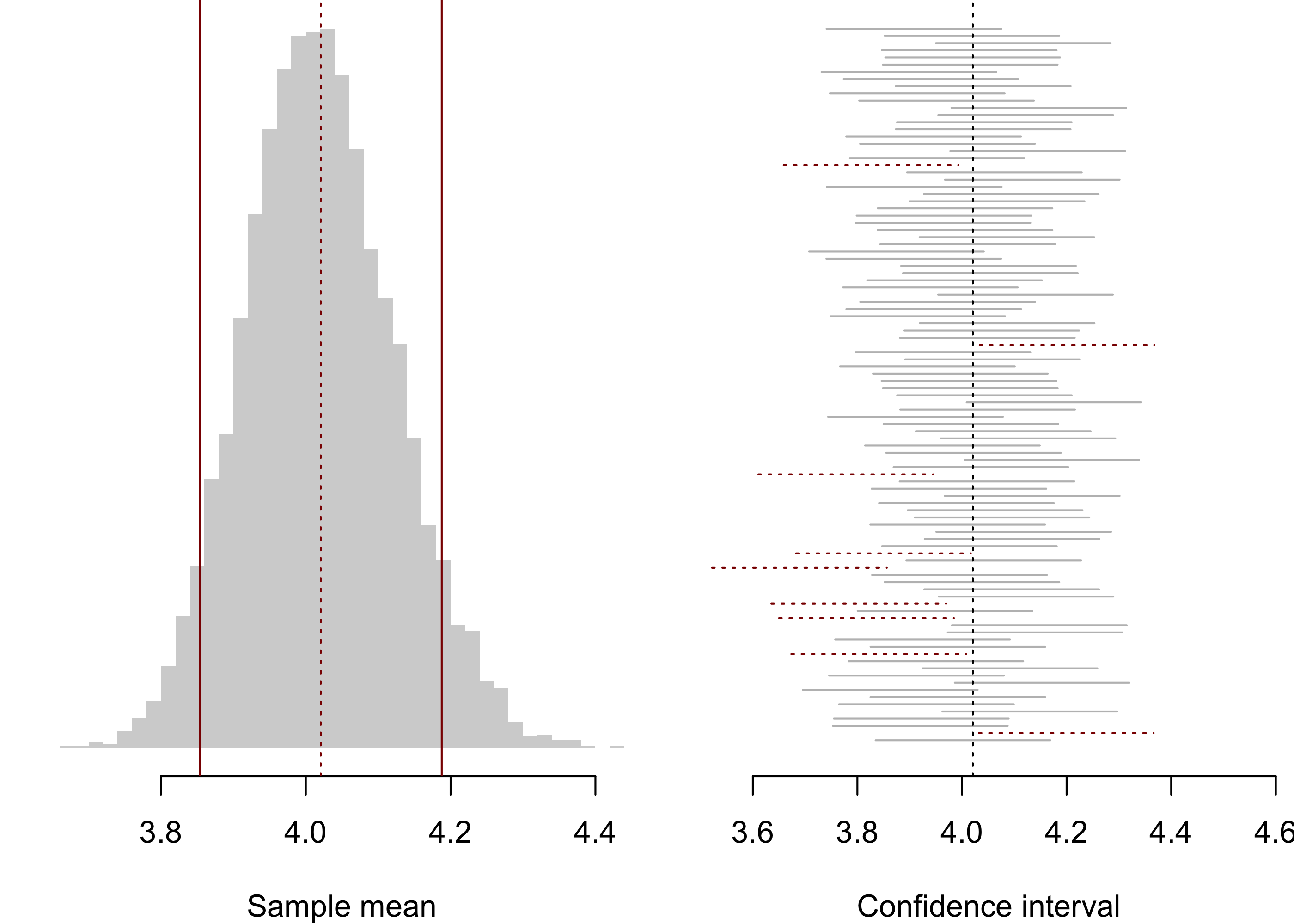
Figure 27.1: Simulation studying the performance of confidence interval \(\bar X_n \pm z_{\alpha/2}\sigma/\sqrt{n}\) treating the distribution of womens finishing times in the 2009 Boston Marathon as the population distribution.

Figure 27.1 shows the results of a simulation study investigating the performance of the confidence interval in Equation 27.1 when the population distribution is non-normal. Treating the distribution of womens finishing times in the 2009 Boston Marathon of Example 17.1 as the population distribution (which has mean \(\mu = 4.021\) and standard deviation \(\sigma = 0.556\) and is a right-skewed distribution), samples of size \(n = 30\) were drawn repeatedly (\(5000\) times) and the confidence interval at \(\alpha = 0.10\) computed. The left panel shows a histogram of the \(\bar X_n\) values with a vertical dotted line indicating the location of the population mean. The value of \(\bar X_n\) must fall between the two solid vertical lines in order that the confidence interval contain \(\mu\). The right panel depicts the first one hundred confidence intervals, each represented as a horizontal line connecting the endpoints. Confidence intervals failing to contain \(\mu\) are represented with dotted lines. Of the \(5000\) samples of size \(n = 30\) drawn, the confidence interval in Equation 27.1 contained \(\mu = 4.021\) a total of \(4478\) times, or \(89.56\%\) of the time. Since \(\alpha = 0.10\) was used, this is fairly close to the advertised \(90\%\) confidence level.

In practice, we will seldom have knowledge of the value of population variance \(\sigma^2\), so we must use the value of \(S_n^2\) as an estimate. In the case of sampling from a normal population, we compensated for the substitution of \(S_n\) for \(\sigma\) by substituting the \(t\) distribution quantile \(t_{n-1,\alpha}\) for the standard normal quantile \(z_{\alpha/2}\). This made the interval wider by just the right amount to ensure that the interval would still cover \(\mu\) with probability \(1-\alpha\). In the case we are considering presently—that of a large sample drawn from a non-normal distribution—there is no principled reason to replace \(z_{\alpha/2}\) with \(t_{n-1,\alpha/2}\), as the quantity \[ \frac{\bar X_n - \mu}{S_n/\sqrt{n}} \] has the \(t_{n-1}\) distribution only when the population distribution is normal. What then, should we do? We find that we can rely on the central limit theorem coupled with a result called Slutzky’s theorem to make the following claim:

Proposition 27.1 (Central limit theorem for Studentized sample mean) If \(X_1,\dots,X_n\) is a random sample from a distribution with mean \(\mu\) and variance \(\sigma^2 < \infty\), then \[ \frac{\bar X_n - \mu}{S_n/\sqrt{n}} \text{ behaves more and more like } Z \sim \mathcal{N}(0,1) \] for larger and larger \(n\).

We can understand the result by writing \[ \frac{\bar X_n - \mu}{S_n/\sqrt{n}} = \frac{\bar X_n - \mu}{\sigma/\sqrt{n}} \frac{\sigma}{S_n} \] and noting that the first factor on the right hand side, by the central limit theorem, behaves more and more like a standard normal random variable for larger and larger \(n\), while the ratio \(\sigma / S_n\), given that \(S_n\) will tend to lie closer and closer to \(\sigma\) for larger and larger \(n\), will be closer and closer to one, so that the effect of substituting \(S_n\) for \(\sigma\) will become negligible; by this reasoning we can see that the entire right hand side should be approximately normally distributed for large enough \(n\).

We may therefore replace \(\sigma\) with \(S_n\) in the interval constructed in Equation 27.1 provided \(n\) is large:

Proposition 27.2 (Large sample confidence interval for a population mean) If \(X_1,\dots,X_n\) is a random sample from distribution with mean \(\mu\) and variance \(\sigma^2<\infty\), then for any \(\alpha \in (0,1)\) the interval with endpoints \[ \bar X_n \pm z_{\alpha/2}\frac{S_n}{\sqrt{n}} \tag{27.2}\] will contain \(\mu\) with probability approximately \(1-\alpha\) for large \(n\).

As a last remark on whether we should not always replace the standard normal quantile \(z_{\alpha/2}\) with the \(t\) distribution quantile \(t_{n-1,\alpha/2}\) whenever replacing \(\sigma\) with \(S_n\), we note that for larger and larger \(n\), the \(t\) distribution quantile \(t_{n-1,\alpha/2}\) becomes closer and closer to \(z_{\alpha/2}\), so it does not really matter, when \(n\) is large, whether one constructs the interval as in Equation 27.2 or as \(\bar X_n \pm t_{n-1,\alpha/2}S_n/\sqrt{n}\).

Xbar <- L <- U <- covered <- numeric(S)
for(s in 1:S){
  
  X <- sample(w,n)
  Xbar[s] <- mean(X)
  M <- za2 * sd(X) / sqrt(n)
  L[s] <- Xbar[s] - M
  U[s] <- Xbar[s] + M

  covered[s] <- (L[s] <= mu) & (U[s] >= mu)
  
}

In a similar situation to that depicted in Figure 27.1, the interval in Equation 27.2, which uses \(S_n\) instead of \(\sigma\), contained \(\mu\) for \(4399\) of the \(5000\) random samples of size \(n=30\), or \(87.98\%\) of the time under \(\alpha = 0.10\), so the performance is seen to be somewhat worse (we are targeting \(90\%\) coverage) when we have to estimate \(\sigma\).

Our rule of thumb will be to require that \(n \geq 30\) before constructing these intervals. Figure 27.2 gives a flow chart.

---
config:
  look: handDrawn
---
flowchart LR
  %% root
  Root["Population distribution"]

  %% bags
  normal["$$\sigma^2$$"]
  nonnormal["$$n$$"]
  

  %% root -> bags (edge labels)
  Root -->|normal|normal
  Root -->|not normal|nonnormal
  
  %% normal leaves
  normal_known["$$\bar X_n \pm z_{\alpha/2}\frac{\sigma}{\sqrt{n}}$$"]
  normal_unknown["$$\bar X_n \pm t_{n-1,\alpha/2}\frac{S_n}{\sqrt{n}}$$"]
  normal -->|known| normal_known
  normal -->|unknown| normal_unknown

  %% nonnormal leaves
  nonnormal_geq30["$$\sigma^2$$"]
  
  nonnormal --> |at least 30|nonnormal_geq30
  nonnormal --> |less than 30|nonnormal_lt30

  nonnormal_geq30_known["$$\bar X_n \pm z_{\alpha/2}\frac{\sigma}{\sqrt{n}}$$"]
  nonnormal_geq30_unknown["$$\bar X_n \pm z_{\alpha/2}\frac{S_n}{\sqrt{n}}$$"]
  

  nonnormal_lt30["Can do nothing so far"]

  nonnormal_geq30 -->|known| nonnormal_geq30_known
  nonnormal_geq30 -->|unknown| nonnormal_geq30_unknown

Figure 27.2: When to build which confidence interval for the population mean.

---

1. The population distribution is not normal, but since the sample size is greater than \(30\), we can treat \(\bar X_n\) like a \(\mathcal{N}(\mu,10/35)\) random variable. For a \(90\%\) confidence interval we have \(\alpha = 0.10\), so we need \(z_{\alpha/2} = z_{0.05}\). We have \(z_{0.05} = 1.645\) (see Figure 13.5). Therefore, a \(90\%\) confidence interval for \(\mu\) is given by \[ 25 \pm 1.645\frac{\sqrt{10}}{\sqrt{35}} = [24.12 , 25.88]. \] We are \(90\%\) confident that the mean \(\mu\) lies within the interval \([24.12 , 25.88 ]\).