22  Normal approximation to the binomial

$$

$$

One additional consequence of applying the central limit theorem to the sample proportion is the so-called normal approximation to the binomial, which we develop here.

For large \(n\), the central limit theorem applied to the mean of a random sample of Bernoulli random variables with success probability \(p\) can be used to claim \[ n \hat p_n \overset{\operatorname{approx}}{\sim}\mathcal{N}(np,np(1-p)), \] where the approximation improves for larger and larger \(n\). We obtain this by multiplying \(\hat p_n\) by \(n\) in Equation 21.1. Now, since \(n \hat p_n \sim \text{Binomial}(n,p)\), it seems that for a Binomial random variable \[ X \sim \text{Binomial}(n,p), \] we should be able to approximate the probabilities \(P(X = x)\) using the \(\mathcal{N}(np,p(1-p)/n)\) distribution. We can do this, but since the Normal distribution is for a continuous random variable, it will assign probability zero to any single value \(x\). To get around this, we note that for the binomial random variable \(X\), which is discrete, we have \[ P(X = x) = P( x - 1/2 < X < x + 1/2) \] for every integer-valued \(x\), so we will approximate the probability \(P(X = x)\) with the probability assigned by the \(\mathcal{N}(np,np(1-p))\) distribution to the interval \((x - 1/2,x+1/2)\). That is, we will use the approximation \[ P(X = x) \approx \left\{\begin{array}{ll}\Phi\Big(\frac{x + 1/2 - np}{\sqrt{np(1-p)}}\Big),& x = 0\\ \Phi\Big(\frac{x + 1/2 - np}{\sqrt{np(1-p)}}\Big) - \Phi\Big(\frac{x - 1/2 - np}{\sqrt{np(1-p)}}\Big),& x > 0, \end{array}\right. \] where \(\Phi\) denotes the CDF of the \(\mathcal{N}(0,1)\) distribution. 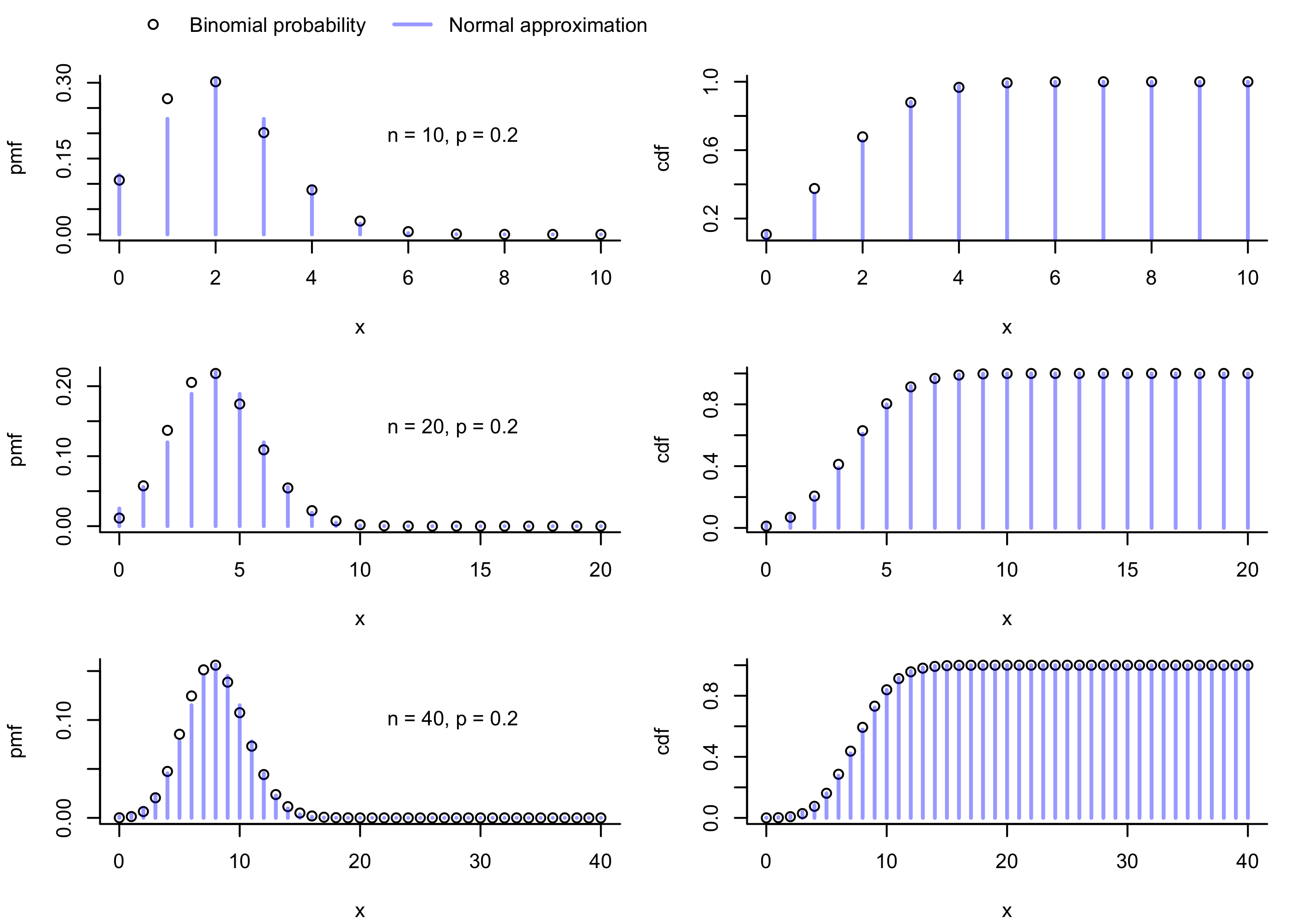Likewise, we will approximate the cumulative distribution function of the \(\text{Binomial}(n,p)\) distribution as \[ P(X \leq x) \approx \Phi\Big(\frac{x + 1/2 - np}{\sqrt{np(1-p)}}\Big) \] These approximations improve with larger and larger \(n\). Figure 22.1 depicts the probabilities \(P(X = x)\) and \(P(X \leq x)\) and their approximations via this method when \(X \sim \text{Binomial}(n,p)\) for the sample sizes \(n = 10,20,40\) with \(p = 0.20\).

p <- 1/5 # success probability
nn <- c(10,20,40) # select a few sample sizes

# set up plotting so the the plots will appear in a 3 by 2 grid
par(mfrow=c(3,2),
    mar=c(4.1,4.1,1.1,1.1), # adjust the margin of each plot so the plots don't get squished
    oma = c(0,0,2,0)) # make a top outer margin in which to place a legend

# loop through the three sample sizes in nn
for(i in 1:3){

  # set sample size for this step in the loop
  n <- nn[i] 
  x <- 0:n
  
  # obtain normal approximations to cdf and pmf
  x_correct <- 0:n + 0.5 # use the continuity correction
  pn <- pnorm(x_correct,n*p,sd = sqrt(n*p*(1-p))) # cdf
  dn <- c(pn[1],diff(pn)) # pmf by differencing. Check ?diff
  
  # make plots
  plot(dbinom(x,n,p)~x,
       bty = "l",
       xlab = "x",
       ylab = "pmf")
  
  points(dn~x, col = rgb(0,0,1,.4), type = "h", lwd = 2)
  
  xpos <- grconvertX(.7,from="nfc",to="user")
  ypos <- grconvertY(.7,from="nfc",to="user")
  
  text(x = xpos, 
       y = ypos,
       labels = paste("n = ",n,", p = ",p,sep=""))

  plot(pbinom(x,n,p)~x,
       bty = "l",
       xlab = "x",
       ylab = "cdf"
       )
  
  points(pn~x, col = rgb(0,0,1,.4), type = "h", lwd = 2)
  
}

xpos <- grconvertX(.1,from="ndc",to="user")
ypos <- grconvertY(1,from="ndc",to="user")
legend(x = xpos, 
       y = ypos,
       horiz = T, # give legend a horizontal orientation
       pch = c(1,NA),
       lty = c(NA,1),
       lwd = c(NA,2),
       col = c("black",rgb(0,0,1,.4)),
       legend = c("Binomial probability",
                  "Normal approximation"),
       bty = "n",
       xpd = NA) # xpd = NA is sometimes need to make something appear in the outer margin

Figure 22.1: Illustration of the normal approximation to the binomial distribution.