ft <- c(2.5692,2.5936,2.6190,2.6320,2.6345,
        2.6602,2.6708,2.6804,2.6850,2.7049,
        2.7111,2.8034,2.8300,3.0639,3.1489,
        3.2411,3.5701,3.9686,4.1220)
xbar <- mean(ft) # sample mean
sn2 <- var(ft)   # sample variance
sn <- sd(ft) # sample standard deviation18 The sample variance
$$
$$
Apart from the mean \(\bar X_n\) of a random sample, another oft-computed sample statistic is the sample variance, which is a description of how spread out the values in the sample are.
Definition 18.1 (Sample variance) For a random sample \(X_1,\dots,X_n\) the sample variance is defined as \[ S^2_n = \frac{1}{n-1}\sum_{i=1}^n(X_i - \bar X_n)^2. \] Moreover \(S_n = \sqrt{S_n^2}\) is called the sample standard deviation.
We can think of the sample variance as the average squared deviation of the values in the sample around the sample mean. One sees that \(S_n^2\) is not a proper average, though, because of division by \(n-1\) instead of \(n\). We will later on give reasons for why the sample variance is defined in this way.
Recall the pinewood derby car data in Example 15.1. The code below reads in the data and computes the sample mean \(\bar X_n\), the sample variance \(S_n^2\), and the sample standard deviation \(S_n\).
We obtain \(\bar X_n = 2.943\), \(S_n^2 = 0.221\), and \(S_n = 0.47\). To report these numbers properly, one really should attach units to them. The values \(X_1,\dots,X_n\) in the random sample are measured in seconds. The sample mean \(\bar X_n\) is therefore also in seconds; however the sample variance, since it is an average of squared deviations from the mean, should be reported as “seconds squared”. The sample standard deviation, since it is the square root of the sample variance, can be reported in the original units. So the sample standard deviation for the pinewood derby car finishing times is \(0.47\) seconds.
Now, the sample variance and sample standard deviation are themselves random variables, as they are computed on the set of random variables \(X_1,\dots,X_n\) comprising the random sample. They therefore have probability distributions of their own. We first consider the expected value the sample variance \(S_n^2\).
Proposition 18.1 (Expected value of the sample variance) If \(X_1,\dots,X_n\) is a random sample from a distribution with variance \(\sigma^2\), then \(\mathbb{E}S_n^2 = \sigma^2\).
We can interpret the above result as saying that if we were to collect a large number, say 1000, of random samples from the same distribution and compute on each one of them the sample variance \(S^2_n\), then the average of all 1000 of these sample variance values should be close to \(\sigma^2\). That is, the sampling distribution of \(S_n^2\) is centered at the population variance \(\sigma^2\).
It turns out that the division by \(n-1\) instead of \(n\) in the definition of the sample variance is necessary for the sampling distribution of \(S_n^2\) to be centered at \(\sigma^2\). If we divide by \(n\) instead of \(n-1\), our the sampling distribution of \(S_n^2\) will have a mean somewhat lower than the population variance \(\sigma^2\). Given that \(S_n^2\) is defined such that \(\mathbb{E}S_n^2 = \sigma^2\), it will be natural to take the value of \(S_n^2\) as a guess for the value of \(\sigma^2\) when the latter is unknown. That is, we will use \(S_n^2\) as an estimator for \(\sigma^2\).
It may be interesting to compute the proportion of the pinewood derby finishing times within one, two, and three sample standard deviations of the sample mean, which may tell us something about whether these data arose from a normal distribution.
p1 <- mean((ft >= xbar - sn) & (ft <= xbar + sn))
p2 <- mean((ft >= xbar - 2*sn) & (ft <= xbar + 2*sn))
p3 <- mean((ft >= xbar - 3*sn) & (ft <= xbar + 3*sn))
We find \(84.211\%\) of the finishing times lie within one sample standard deviations of \(\bar X_n\), \(89.474\%\) lie withing two sample standard deviations of \(\bar X_n\), and \(100\%\) lie within three sample standard deviations of \(\bar X_n\). Figure 18.1 shows a histogram of the pinewood derby finishing times with regions delineating one, two, and three sample standard devations \(S_n\) from the sample mean \(\bar X_n\). We see from this plot that the distribution of finishing times is far from symmetric.
Code
import numpy as np
import matplotlib.pyplot as plt

plt.rcParams['figure.dpi'] = 128
plt.rcParams['savefig.dpi'] = 128
plt.rcParams['figure.figsize'] = (7, 4)

X = np.array([2.5692,2.5936,2.6190,2.6320,2.6345,2.6602,
              2.6708,2.6804,2.6850,2.7049,2.7111,2.8034,
              2.8300,3.0639,3.1489,3.2411,3.5701,3.9686,
              4.1220])

n = X.size
Xbar = np.mean(X)
Sn = np.std(X)*np.sqrt(n/(n-1))

fig, ax = plt.subplots()


ax.fill([Xbar - 3*Sn,Xbar - 3*Sn,Xbar + 3*Sn,Xbar + 3*Sn],[-1,10,10,-1],'gainsboro')
ax.fill([Xbar - 2*Sn,Xbar - 2*Sn,Xbar + 2*Sn,Xbar + 2*Sn],[-1,10,10,-1],'lightgray')
ax.fill([Xbar - Sn,Xbar - Sn,Xbar + Sn,Xbar + Sn],[-1,10,10,-1],'lightsteelblue')


ax.hist(X,density = True)

ax.set_ylim([0,4]);
ax.set_xlabel('Finishing times')
ax.set_ylabel('Density')


plt.show()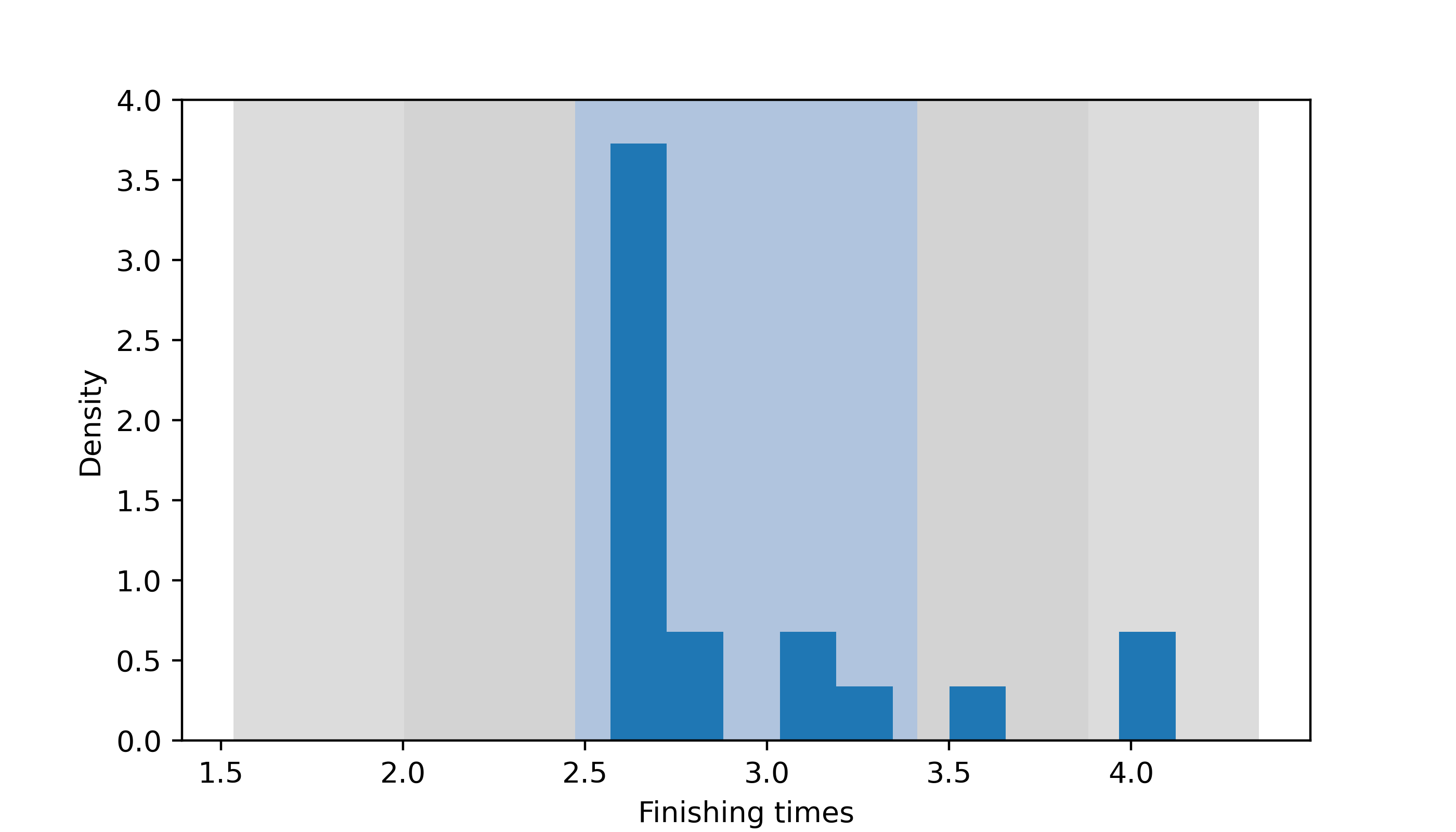
We will have more to say about the distribution of the sample variance \(S_n^2\) later on. Specifically, we will learn that if we scale it as \((n-1)S_n^2/\sigma^2\), this will have a distribution called a chi-squared distribution.