A problem central to nonparametric statistics is how to estimate a probability density function \(f\) from a sample of independent realizations \(X_1,\dots,X_n\) of a random variable \(X \sim f\). If one assumes \(f\) belongs to a parametric family such that \(f(\cdot) = f(\cdot ; \boldsymbol{\theta})\) for a set of parameters \(\boldsymbol{\theta}= (\theta_1,\dots,\theta_d) \in \Theta \subset \mathbb{R}^d\) for some finite \(d \geq 1\), then one could estimate \(f\) by estimating the parameters in \(\boldsymbol{\theta}\). That is, one could estimate \(f(\cdot)\) with \(f(\cdot;\hat{\boldsymbol{\theta}})\), where \(\hat{\boldsymbol{\theta}}\) is an estimator of \(\boldsymbol{\theta}\).
For example, we might assume \[
f(x) = f(x;\boldsymbol{\theta}) = \frac{1}{\Gamma(\theta_1)\theta_2^{\theta_1}}x^{\theta_1 - 1}e^{-x/\theta_2}\mathbf{1}(x > 0)
\] for all \(x \in \mathbb{R}\), where \(\boldsymbol{\theta}= (\theta_1,\theta_2)\), i.e. that \(X\) has the gamma distribution with mean \(\theta_1\theta_2\) and variance \(\theta_1\theta_2^2\). Then we could estimate \(f(x)\) with \(f(x;\hat{\boldsymbol{\theta}})\), where \(\hat{\boldsymbol{\theta}} = (\hat \theta_1,\hat \theta_2)\) and \(\hat \theta_1\) and \(\hat \theta_2\) are, say, the maximum likelihood estimators of \(\theta_1\) and \(\theta_2\).
In nonparametric statistics we wish to estimate \(f\) without assuming it belongs to any particular parametric family. We have already discussed estimation of the cumulative distribution function (cdf) \(F\) with the empirical cdf \[
\hat F_n(x) = \frac{1}{n}\sum_{i=1}^n \mathbf{1}(X_i \leq x).
\] The first nonparametric estimator of \(f\) we will discuss is the so-called Rosenblatt estimator, which uses the fact if \(F\) is differentiable, the density \(f\) is equal to the derivative of \(F\). Using the definition of the derivative as a limit, we may write \[
f(x) = \frac{d}{dx}F(x) = \lim_{h\to 0}\frac{F(x + h) - F(x)}{h}.
\] Note that we can also write the derivative as \[
f(x) = \lim_{h\to 0} \frac{F(x + h) - F(x - h)}{2h}.
\] This formula motivates the Rosenblatt estimator; the estimator is constructed by replacing \(F\) in the above expression by \(\hat F_n\) and fixing \(h\) at some small value. Thus set \[
\hat f_{n,h}^R(x) =\frac{\hat F_n(x + h) - \hat F_n(x - h)}{2h}
\] for all \(x \in \mathbb{R}\) for some small \(h > 0\).
The Rosenblatt estimator is a special case of a type of estimator called a kernel density estimator of a pdf.
Definition 1.1 (Kernel density estimator) A kernel density estimator (KDE) takes the form \[
\hat f_{n,h}(x) = \frac{1}{nh}\sum_{i=1}^nK\Big(\frac{X_i - x}{h}\Big),
\tag{1.1}\] where the function \(K(\cdot)\) is called the kernel and \(h > 0\) is called the bandwidth.
Note that we may write \[\begin{align*}
\hat f_{n,h}^R(x) &=\frac{\hat F_n(x + h) - \hat F_n(x - h)}{2h} \\
&=\frac{1}{2nh}\sum_{i=1}^n\mathbf{1}(x -h \leq X_i \leq x + h) \\
&=\frac{1}{nh}\sum_{i=1}^n\frac{1}{2}\mathbf{1}\Big(-1 \leq \frac{X_i - x}{h} \leq 1\Big),
\end{align*}\] which has the form of the KDE \(\hat f_{n,h}(x)\) in Equation 1.1 with kernel \(K(\cdot)\) given by \(K(u) = (1/2)\mathbf{1}(-1 \leq u \leq 1)\). We may refer to this kernel as the Rosenblatt kernel.
Some kernels found in the literature are:
The triangular kernel \(K(u) = (1 - |u|)\mathbf{1}(|u|\leq 1)\).
The Epanechnikov kernel \(K(u) = (3/4)(1 - u^2)\mathbf{1}(|u|\leq1)\).
The Gaussian kernel \(K(u) = (2\pi)^{-1/2}e^{-u^2/2}\).
The Silverman kernel \(K(u) = (1/2)e^{-|u|/2}\sin(|u|/\sqrt{2} + \pi/4)\).
One may wonder what kinds of functions are suitable as kernels in a KDE. If one wishes the KDE \(\hat f_n\) to be a valid probability density function, i.e. that \(\hat f_{n,h}(x) \geq 0\) for all \(x\in \mathbb{R}\) and \(\int_\mathbb{R}\hat f_{n,h}(x)dx = 1\), one can guarantee this by selecting a kernel \(K\) which is itself a density.
Proposition 1.1 (Conditions on the kernel for the KDE to be a valid density) If \(K\) is a density then \(\hat f_{n,h}\) is a density.
Let \(K\) be a density. Then \(K(u) \geq 0\) for all \(u \in \mathbb{R}\), so \(\hat f_n(x) \geq 0\) for all \(x \in \mathbb{R}\). Moreover \[\begin{align*}
\int_\mathbb{R}\hat f_{n,h}(x)dx &= \frac{1}{nh} \sum_{i=1}^n \int_\mathbb{R}K\Big(\frac{X_i - x}{h}\Big)dx \\
&= \frac{1}{nh} \sum_{i=1}^n \int_\infty^{-\infty} K(u)(-h)du \quad \text{ sub } u = (X_i - x)/h\\
&= \int_{-\infty}^\infty K(u)du\\
&= 1,
\end{align*}\] so \(\hat f_{n,h}\) is a density.
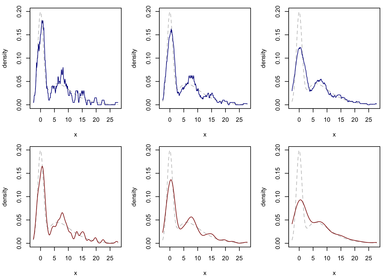
Figure Figure 1.1 shows KDEs with the Rosenblatt and Gaussian kernels computed on a sample of size \(n = 200\) at three different choices of the bandwidth. The true density from which the data were drawn is overlaid in each plot. One notes that the Gaussian kernel is rather more pleasing to the eye.
Code
# draw a random sample from a mixture distributionn <-200d <-sample(c(0,1),n,replace=TRUE)Y <- d *rgamma(n,3,scale =3) + (1- d) *rnorm(n)# define a sequence of x values over which to compute the KDEsmin <-qnorm(.005)max <-qgamma(.995,3,scale =3)x <-seq(min,max,length =300)# compute the value of the true density over the values of xfx <-dgamma(x,3,scale =3) *1/2+dnorm(x) *1/2# define a function to compute the KDE at a point xkde <-function(x,Y,h,K = dnorm) mean(K((Y-x)/h)) / h# compute two kdes at each of three bandwidthshh <-c(0.5,1,2)kde_gauss_x <-matrix(0,length(x),length(hh))kde_rosenblatt_x <-matrix(0,length(x),length(hh))for(j in1:length(hh)){ kde_gauss_x[,j] <-sapply(X = x, FUN = kde, Y = Y, h = hh[j]) kde_rosenblatt_x[,j] <-sapply(X = x, FUN = kde, Y = Y, h = hh[j], K =function(u){(abs(u) <=1) /2}) }par(mfrow =c(2,3), mar =c(4.1,4.1,1.1,1.1))ylims <-range(fx,kde_gauss_x,kde_rosenblatt_x)for(j in1:length(hh)){plot(fx~x,type ="l",ylim = ylims,xlab ="x",ylab ="density",lty =2,col ="gray")lines(kde_rosenblatt_x[,j]~ x, col =rgb(0,0,.545))}for(j in1:length(hh)){plot(fx~x,type ="l",ylim = ylims,xlab ="x",ylab ="density",lty =2,col ="gray")lines(kde_gauss_x[,j]~ x, col =rgb(0.545,0,0))}
Figure 1.1: Top: Rosenblatt KDE with bandwidth increasing from left to right. Bottom: Gaussian KDE with bandwidth increasing from left to right. True density shown in each plot.