In our preparation to discuss minimax theory, we have drawn, in the last section, a connection between nonparametric regression and the Normal means model. This is because it is simpler to present minimax results in terms of the Normal means model than in a general nonparametric regression setting.
We now introduce a class of functions called periodic Xobolev functions, which is perhaps the class of functions most amenable to minimax analysis via the Normal means model.
Definition 22.1 For \(\beta\) a positive integer and \(L > 0\), define the Sobolev class of functions \(\mathcal{W}(\beta,L)\) as \[
\mathcal{W}(\beta,L) = \Bigg\{m : [0,1] \to \mathbb{R}: \quad \begin{array}{l}
m^{(\beta-1)} \text{ is absolutely continuous }\\
\text{ and }\int_0^1|m^{(\beta)}(x)|^2dx \leq L\end{array}\Bigg\}.
\] Moreover, define the periodic Sobolev class \(\mathcal{W}_\text{per}(\beta,L)\) as \[
\mathcal{W}_\text{per}(\beta,L) = \Big\{m \in \mathcal{W}(\beta,L): \quad m^{(j)}(0) = m^{(j)}(1), \quad j = 1,\dots,\beta\Big\}.
\]
We find we can construct all the functions in a periodic Sobolev class from the Fourier basis such that the coefficients \(\theta_1,\theta_2,\dots\) lie in an ellipsoid called a Sobolev ellipsoid.
Definition 22.2 (Sobolev ellipsoid) Define the Sobolev ellipsoid \(\Theta(\beta,c)\) as \[
\Theta_{\text{Sob}}(\beta,L) = \Big\{(\theta_1,\theta_2,\dots) \in \mathbb{R}: \quad \sum_{j=1}^\infty \theta^2_j < \infty \text{ and } \sum_{j=1}^\infty a_j^2 \theta_j^2 \leq L^2/\pi^{2\beta}\Big\},
\] where \[
a_j = \left\{\begin{array}{ll}
j^\beta,& j \text{ even}\\
(j-1)^\beta,& j \text{ odd}
\end{array}\right.
\] for \(j = 1,2,\dots\)
The next result is adapted from Proposition 1.14 on page 50 of Tsybakov (2008).
Theorem 22.1 (Basis for periodic Sobolev functions) We have \[
\mathcal{W}_{\text{per}}(\beta,L) = \Big\{ m : \quad m(x) = \sum_{j=1}^\infty \theta_j \varphi_j(x),\quad (\theta_1,\theta_2,\dots) \in \Theta_{\text{Sob}}(\beta,L)\Big\},
\] where \(\varphi_1,\varphi_2,\dots\) is the Fourier basis.
So, to understand how well we can estimate functions belonging to a periodic Sobolev class, we can study how well we can estimate \(\theta_1,\theta_2,\dots\) in the Normal means model when the unknown parameters lie in a Sobolev ellipsoid.
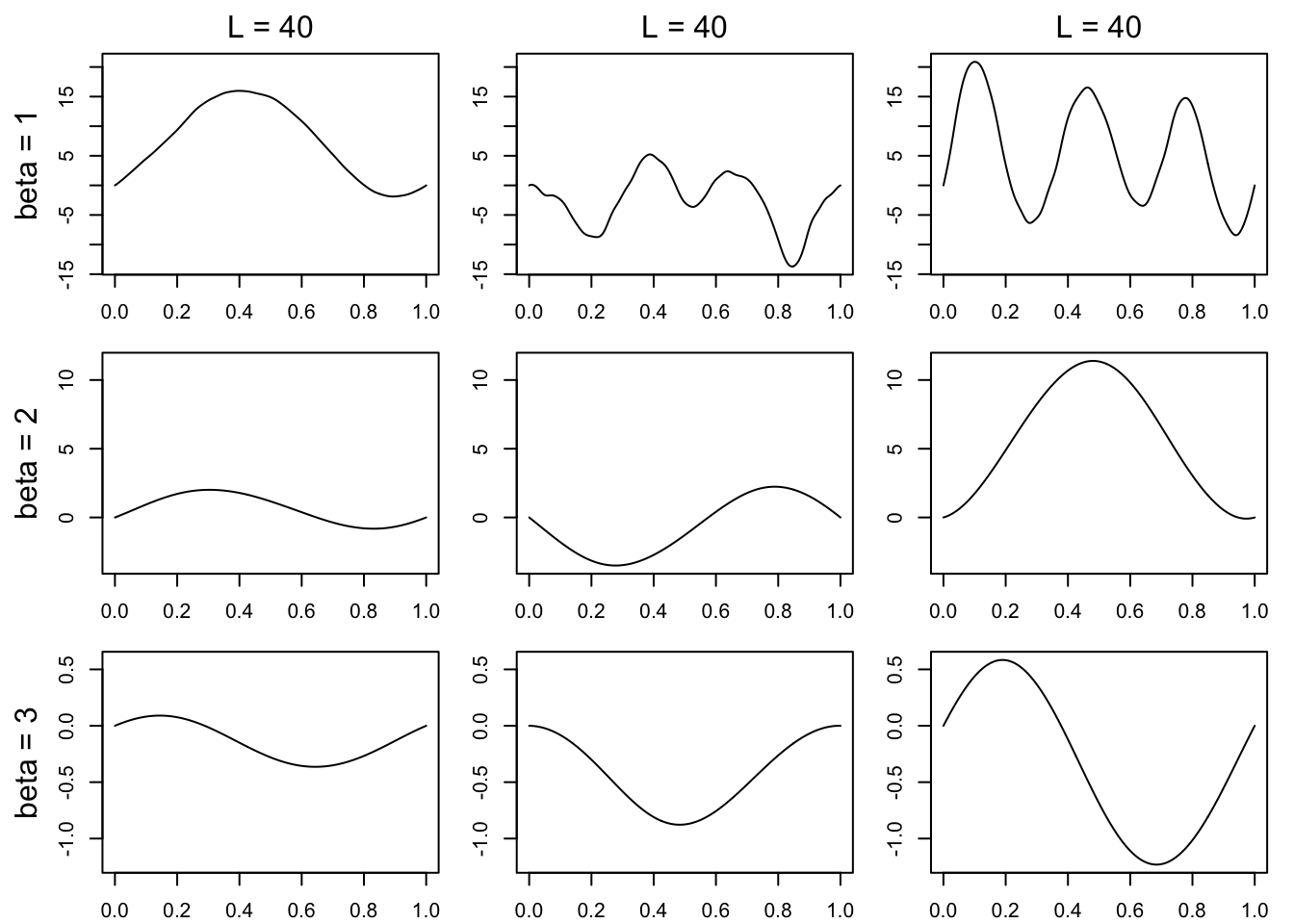
Figure 22.1 shows some functions from periodic Sobolev classes \(\mathcal{W}_\text{per}(\beta,L)\) for a few combinations of \(\beta\) and \(L\) values. The functions are randomly selected in these steps:
Draw \(\theta_1,\dots \theta_N \overset{\text{ind}}{\sim}\mathcal{N}(0,1)\) with \(N = 50\).
Minimize \(\sum_{i=1}^N(\theta_j - w_j)^2\) subject to \(\sum_{j = 1}^N a_j^2w_j^2 = L^2/\pi^{2\beta}\), where the \(a_j\) are those which define the Sobolev ellipsoid \(\Theta_{\text{Sob}}(\beta,L)\).
Set \(m(x) = \sum_{j=1}^N\hat w_j \varphi_j(x)\), where \(\hat w_1,\dots,\hat w_N\) are from Step 2 and \(\varphi_1,\varphi_2,\dots\) is the Fourier basis.
Figure 22.1: Some randomly selected functions from periodic Sobolev classes \(\mathcal{W}_\text{per}(\beta,L)\). Each is centered such that \(m(0) = 0\).
Note that the functions become smoother for larger \(\beta\) and have less variation for smaller \(L\).
Next we will consider finding the minimax rate for estimating \(\theta_1,\theta_2,\dots\) in the Normal means model when the unknown parameters lie in a Sobolev ellipsoid.
Tsybakov, Alexandre B. 2008. Introduction to Nonparametric Estimation. Springer Science & Business Media.