4 Mean integrated squared error and crossvalidation

Now we consider the selection of the bandwidth \(h\). While various methods for selecting \(h\) have been proposed, we will present a crossvalidation approach, following closely Section 1.4 of Tsybakov (2008). In particular, we will select \(h\) which minimizes an estimate, obtained via a method called crossvalidation, of the mean integrated squared error (MISE) of the kernel density estimator (KDE) \(\hat f_{n,h}(x)\), where the MISE is defined as \[ \operatorname{MISE}\hat f_{n,h} = \mathbb{E}\int_\mathbb{R}[\hat f_{n,h}(x) - f(x)]^2dx. \] Crossvalidation typically involves leaving out one or more observations from the data and computing an estimator on the remaining data, after which one checks how will the estimator “performs” in modeling or predicting the observations which were left out. We will define an estimator of \(\operatorname{MISE}\{\hat f_{n,h} \}\) based on leave-one-out crossvalidation, which will will minimize over a set of candidate bandwidth choices \(h\). To this end, define leave-one-out estimators of \(f(x)\) as \[ \hat f_{n,h,-i}(x) = \frac{1}{(n-1)h}\sum_{j \neq i} K\Big(\frac{X_j - x}{h}\Big), \quad x \in\mathbb{R}, \] for \(i =1,\dots,n\), where each of these is the KDE of \(f(x)\) after removing one observation from among \(X_1,\dots,X_n\).

To understand how the leave-one-out versions of \(\hat f_{n,h}\) can be used to estimate \(\operatorname{MISE}\{\hat f_{n,h} \}\), note that we can decompose the latter as \[ \operatorname{MISE}\hat f_{n,h} = \mathbb{E}\int_\mathbb{R}\hat f_{n,h}^2(x) dx - 2 \mathbb{E}\int_\mathbb{R}\hat f_{n,h}(x)f(x)dx - \int_\mathbb{R}f^2(x)dx, \tag{4.1}\] where only the first two terms involve the bandwidth \(h\). We find we can use the leave-one-out versions of \(\hat f_{n,h}\) to estimate the second term. In particular, we have \[ \mathbb{E}\frac{1}{n}\sum_{i=1}^n \hat f_{n,h,-i}(X_i) = \mathbb{E}\int_\mathbb{R}\hat f_{n,h}(x)f(x)dx, \tag{4.2}\] where, for each \(i\), we have plugged the left-out observation \(X_i\) back into the leave-one-out estimator \(\hat f_{n,h,-i}\) obtained without this observation, and then computed the mean of these evaluations.

Derivation of Equation 4.2

We may write \[\begin{align*} \mathbb{E}\frac{1}{n}\sum_{i=1}^n \hat f_{n,h,-i}(X_i) &= \frac{1}{n}\sum_{i=1}^n \frac{1}{(n-1)h}\sum_{j \neq i} \mathbb{E}K\Big(\frac{X_j - X_i}{h}\Big)\\ &= \frac{1}{h} \mathbb{E}K\Big(\frac{X_1 - X_2}{h}\Big) \\ &= \frac{1}{h} \int_\mathbb{R}\int_\mathbb{R}K\Big(\frac{x - z}{h}\Big)f(z)f(x)dzdx. \end{align*}\] At the same time we have also \[\begin{align*} \mathbb{E}\int_\mathbb{R}\hat f_{n,h}(x)f(x)dx &= \mathbb{E}\int_\mathbb{R}\frac{1}{nh}\sum_{i=1}^nK\Big(\frac{X_i - x}{h}\Big)f(x)dx \\ &=\frac{1}{h} \int_\mathbb{R}\int_\mathbb{R}K\Big(\frac{x - z}{h}\Big)f(z)f(x)dzdx. \end{align*}\] So, provided this integral is finite, Equation 4.2 holds.

Further noting that the realized value of \(\int_\mathbb{R}\hat f_{n,h}^2(x) dx\) is an unbiased estimator for its own expected value (a random variable \(X\) is trivially an unbiased estimator of \(\mathbb{E}X\)), we define \[ \operatorname{CV}_n(h) = \int_\mathbb{R}\hat f_{n,h}^2(x)dx - \frac{2}{n}\sum_{i=1}^n \hat f_{n,h,-i}(X_i), \] for which we have the following result:

Theorem 4.1 (Leave-one-out crossvalidation for KDE bandwidth selection) Provided \(\int_\mathbb{R}f^2(x)dx < \infty\) and \[ \int_\mathbb{R}\int_\mathbb{R}\Big|K\Big(\frac{z-x}{h}\Big)\Big|f(z)f(x)dzdx < \infty \] for all \(h > 0\). Then for all \(h>0\) we have \[ \mathbb{E}\operatorname{CV}_n(h) = \operatorname{MISE}\hat f_{n,h} + \int_\mathbb{R}f^2(x)dx. \]

Theorem 4.1 follows from Equation 4.2 and Equation 4.1 and suggests selecting \(h\) as \[ \hat h_{\operatorname{CV}}= \operatorname{argmin}_{h > 0} \operatorname{CV}_n(h). \]

Code

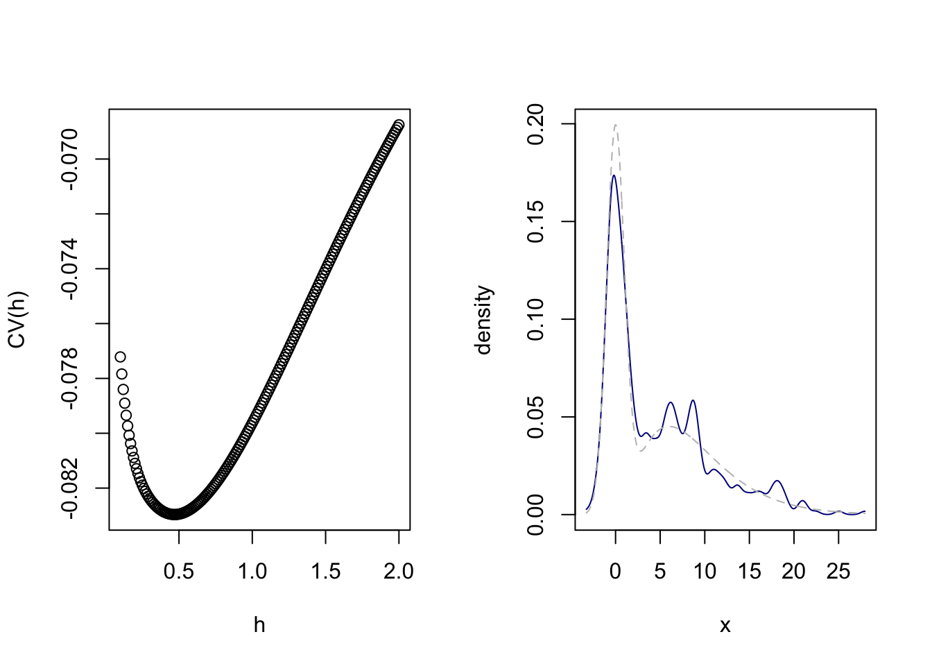
# define the true density function
f <- function(x) dgamma(x,3,scale = 3) * 1/2 + dnorm(x) * 1/2

# draw a sample from a distribution with density f
n <- 500
d <- sample(c(0,1),n,replace=TRUE)
Y <- d * rgamma(n,3,scale = 3) + (1 - d) * rnorm(n)

# define a function to compute the KDE at a point x
kde <- function(x,Y,h,K = dnorm) mean(K((Y-x)/h)) / h
  
# crossvalidation
hh <- seq(0.1,2,by = 0.01)
CV <- numeric(length(hh))
x <- seq(min(Y),max(Y),length=1000) # a range over which to integrate
for(j in 1:length(hh)){
  
  fx <- sapply(x,FUN=kde, Y = Y, h = hh[j])
  A <- sum(fx^2)*(x[2]-x[1]) # numerical integration
  
  B <- 0
  for(i in 1:n) B <- B + kde(Y[i],Y[-i],hh[j]) / n
  
  CV[j] <- A - 2*B

}


par(mfrow = c(1,2))
plot(CV~hh,
     xlab = "h",
     ylab = "CV(h)")
hcv <- hh[which.min(CV)]

# plot kde with crossvalidation choice of h
fx <- sapply(x,FUN=kde, Y = Y, h = hcv)
plot(fx~x,
     type="l",
     ylim = range(f(x),fx), 
     col = rgb(0,0,.545),
     ylab = "density")
lines(f(x)~x,lty=2, col = "gray")

Plot with two panels, one showing a curve with a minimum, the other showing a density with a kernel density estimate overlaid. — Figure 4.1: Left: Crossvalidation to select the bandwidth \(h\). Right: The KDE with bandwidth chosen by crossvalidation.

It is difficult to obtain results giving the performance of the estimator \(\hat f_{n,h}\) under the choice of bandwidth \(h = \hat h_{\operatorname{CV}}\). Specifically, the size of \(\hat h_{\operatorname{CV}}\) with respect to \(n\) as \(n \to \infty\) is not immediately clear.

Here, we considered bandwidth selection with a view to minimizing \(\operatorname{MISE}\hat f_{n,h}\), where we introduced the latter quantity in this section for this purpose. However, one may be interested in analyzing \(\operatorname{MISE}\hat f_{n,h}\) even outside the context of bandwidth selection. In particular, one may be interested in obtaining bounds for \(\operatorname{MISE}\hat f_{n,h}\) analogous to those we have obtained for \(\operatorname{MSE}\hat f_{n,h}(x)\) in previous sections, which is undertaken in Section 1.2.3 of Tsybakov (2008).