Backfitting is a simple and fast algorithm for computing estimators of \(m_1,\dots,m_p\) in the additive model.
To understand the backfitting algorithm, consider more a moment a tuple of random variables \((X_1,\dots,X_p,Y) \in [0,1]^p\times\mathbb{R}\) such that \[
Y = m_1(X_1) + \dots + m_p(X_p) + \varepsilon,
\] where \(\varepsilon\) is independent of \(X_1,\dots,X_p\) and has mean \(0\). Then we may write \[
m_j(X_j) = \mathbb{E}[Y|X_j] - \sum_{k\neq j}\mathbb{E}[m_k(X_k)|X_j]
\] for \(j=1,\dots,p\). Now, if we let \(\Pi_j\) represent the operator which takes the conditional expectation \(\mathbb{E}[ \cdot | X_j]\), and if we write \(m_j(X_j)\) as simply \(m_j\), we can represent the above system of equations symbolically as \[
\left[\begin{array}{cccc}
I&\Pi_1& \dots & \Pi_1 \\
\Pi_2& I & \dots & \Pi_2\\
\vdots & \vdots& \ddots & \vdots \\
\Pi_p & \Pi_p & \dots & I
\end{array}\right] \left[\begin{array}{c}
m_1 \\
m_2\\
\vdots \\
m_p
\end{array}\right] = \left[\begin{array}{c}
\Pi_1 Y \\
\Pi_2 Y\\
\vdots \\
\Pi_p Y
\end{array}\right],
\] where \(I\) is the identity operator (such that \(I m_j = m_j\)).
The strategy of backfitting is to solve an empirical version of this system of equations. Let
\(\mathbf{S}_1,\dots,\mathbf{S}_p\) be \(n \times n\) smoother matrices (Link to the definition of a smoother matrix) associated with univariate smoothers.
\(\mathbf{Y}= (Y_1,\dots,Y_n)^T\) be the \(n\times 1\) vector of response values.
for \(\hat{\mathbf{m}}_1,\dots,\hat{\mathbf{m}}_p\) using the Gauss-Seidel method (see Buja, Hastie, and Tibshirani (1989)). These vectors are \(n\times 1\) vectors, the entries of which are the evaluations of the estimated additive components at the design points. That is \(\hat{\mathbf{m}}_j = (\hat m_j(x_{1j}),\dots,\hat m_j(x_{nj}))^T\) for \(j = 1,\dots,p\).
The steps of the backfitting algoritm are as follows:
Definition 17.1 (Backfitting algorithm) Initialize \(\hat{\mathbf{m}}_1,\dots,\hat{\mathbf{m}}_p = \mathbf{0}\). Then do: For \(j =1,\dots,p\) update \(\hat{\mathbf{m}}_j\) as
until convergence (until the change in \(\hat{\mathbf{m}}_1,\dots,\hat{\mathbf{m}}_p\) is negligible).
To implement the backfitting algorithm, we just need construct the smoother matrices, for example:
Least-squares splines: \(\mathbf{S}_j = \mathbf{B}_j(\mathbf{B}_j^T\mathbf{B}_j)^{-1}\mathbf{B}_j^T\), where \(\mathbf{B}_j = (b_{k}(x_{ij}))_{1\leq i \leq n, 1 \leq k \leq d}\) for \(j=1,\dots,p\), where \(b_1,\dots,b_d\) are, say, cubic B-spline basis functions.
Penalized splines: \(\mathbf{S}_j = \mathbf{B}_j(\mathbf{B}_j^T\mathbf{B}_j + \lambda \boldsymbol{\Omega})^{-1}\mathbf{B}_j^T\) for \(j=1,\dots,p\), where \(\boldsymbol{\Omega}= (\int_0^1b''_k(x)b''_{k'}(x)dx)_{1\leq k,k' \leq d}\) and \(\lambda > 0\) tunes the smoothness.
Nadaraya-Watson: \(\mathbf{S}_j = \left( \dfrac{K((x_{i'j} - x_{ij})/h)}{\sum_{k=1}^nK((x_{k j} - x_{ij})/h)}\right)_{1 \leq i \leq n, 1 \leq i' \leq n}\) for each \(j=1,\dots,p\).
The following code uses the backfitting estimator to estimate each \(m_j\) in an additive model with data generated in a setup considered in Meier et al. (2009).
Code
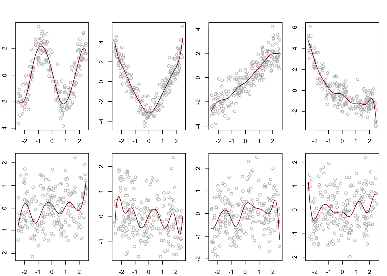
# generate datap <-8rho <-0.5n <-200m1 <-function(x){-2*sin(x*2)}m2 <-function(x){x^2-25/12}m3 <-function(x){x}m4 <-function(x){(exp(-x)-2/5*sinh(5/2))/2}# generate covariates marginally uniform and having correlation matrix RR <- rho^abs( outer(1:p,1:p,"-"))P <-2*sin( R * pi /6)X <- (pnorm( matrix(rnorm(n*p),ncol = p) %*%chol(P)) - .5) *5# make the true functions satisfy the identifiability conditionm1X <-m1(X[,1]) -mean(m1(X[,1]))m2X <-m2(X[,2]) -mean(m2(X[,2]))m3X <-m3(X[,3]) -mean(m3(X[,3]))m4X <-m4(X[,4]) -mean(m4(X[,4]))mu <-4Y <- mu + m1X + m2X + m3X + m4X +rnorm(n,0,1)# build smoother matrices for least-squares splineslibrary(splines)K <-8d <- K +3# number of functionsu <- ((0:K)/K -1/2)*5urep <-c(rep(u[1],3),u,rep(u[K+1],3)) # knotsS <-array(0,dim=c(n,n,p)) # store smoother matrices in an arrayfor(j in1:p){ B <-splineDesign(knots = urep, x = X[,j], ord =3+1) S[,,j] <- B %*%solve(t(B) %*% B) %*%t(B)}# define backfitting functionbackfit <-function(Y,S,tol=1e-6){ n <-length(Y) p <-dim(S)[3] conv <-FALSE M <-matrix(0,n,p)while(conv ==FALSE){ M0 <- Mfor(j in1:p){ M[,j] <- S[,,j] %*% (Y -apply(M[,-j],1,sum)) M[,j] <- M[,j] -mean(M[,j]) } conv <-max(abs(M - M0)) < tol }return(M)}# center the response and obtain the backfitting estimatesYcent <- Y -mean(Y)M <-backfit(Ycent,S)par(mfrow =c(2,4), mar =c(2.1,2.1,1.1,1.1),oma =c(0,0,2,0))for(j in1:p){ Yj <- Ycent -apply(M[,-j],1,sum)plot(Yj ~ X[,j],col ="gray")lines(M[order(X[,j]),j]~sort(X[,j]), col =rgb(.545,0,0))}
Backfitting estimators of additive components using least-squares spline smoothers
Code
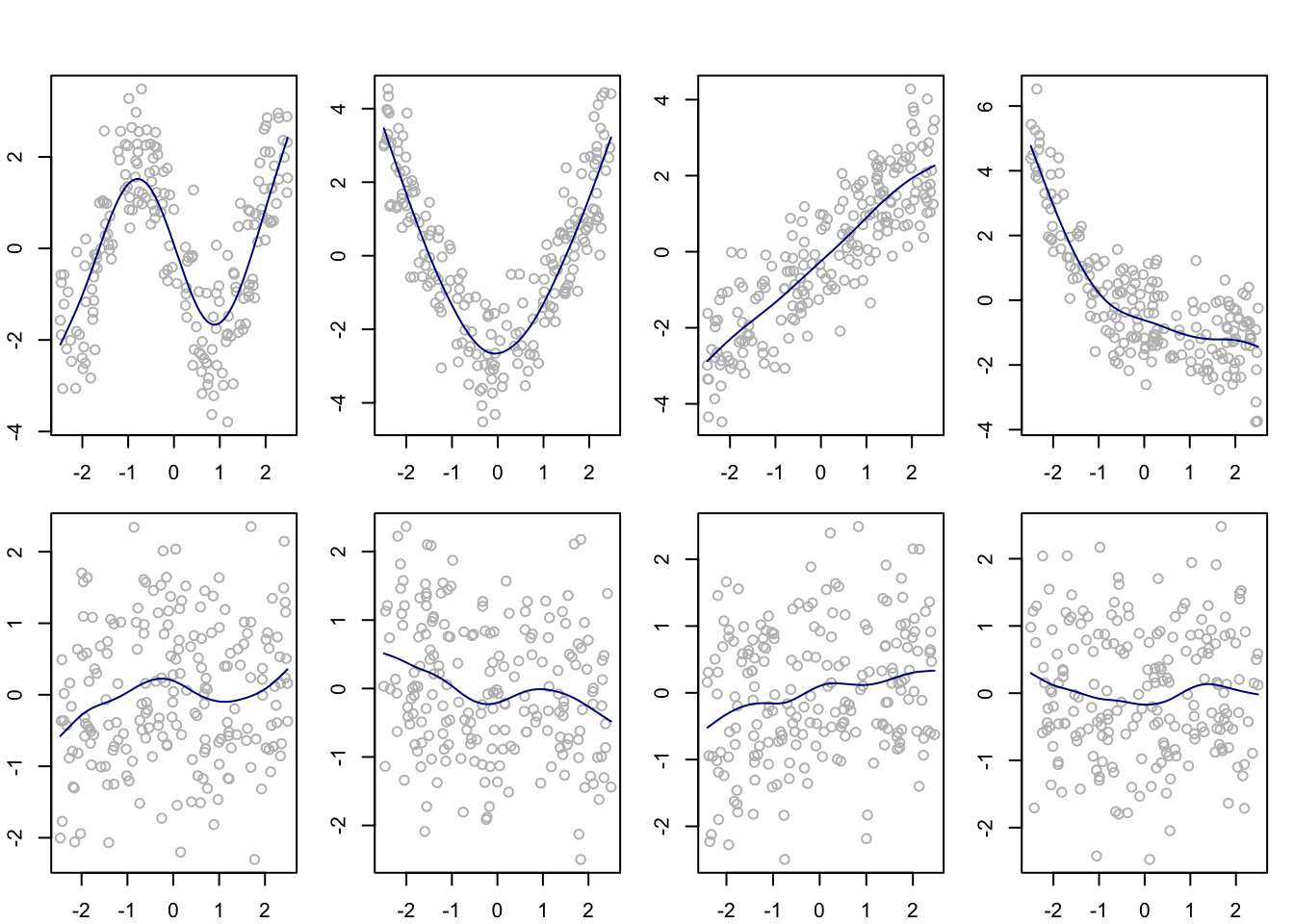
K <-20lam <-1d <- K +3# number of functionsu <- ((0:K)/K -1/2)*5urep <-c(rep(u[1],3),u,rep(u[K+1],3)) # knots# obtain 2nd derivativesddBu <-spline.des(knots = urep,x = u,derivs =rep(2,length(u)),ord =4)$design# compute the matrix OmegaOm <-matrix(NA,K+3,K+3)for(l in1:(K+3))for(j in1:(K+3)){ tk <- ddBu[-(K+1),l] gk <- ddBu[-(K+1),j] tkp1 <- ddBu[-1,l] gkp1 <- ddBu[-1,j] Om[l,j] <-sum((u[-1]-u[-(K+1)])*((1/2)*(gk*tkp1+gkp1*tk)+(1/3)*(tkp1-tk)*(gkp1-gk))) }Spen <-array(0,dim=c(n,n,p)) # store smoother matrices in an arrayfor(j in1:p){ B <-splineDesign(knots = urep, x = X[,j], ord =3+1) Spen[,,j] <- B %*%solve(t(B) %*% B + lam * Om) %*%t(B)}# center the response and obtain the backfitting estimatesYcent <- Y -mean(Y)M <-backfit(Ycent,Spen)par(mfrow =c(2,4), mar =c(2.1,2.1,1.1,1.1),oma =c(0,0,2,0))for(j in1:p){ Yj <- Ycent -apply(M[,-j],1,sum)plot(Yj ~ X[,j],col ="gray")lines(M[order(X[,j]),j]~sort(X[,j]), col =rgb(0,0,.545))}
Backfitting estimators of additive components using penalized spline smoothers
Code
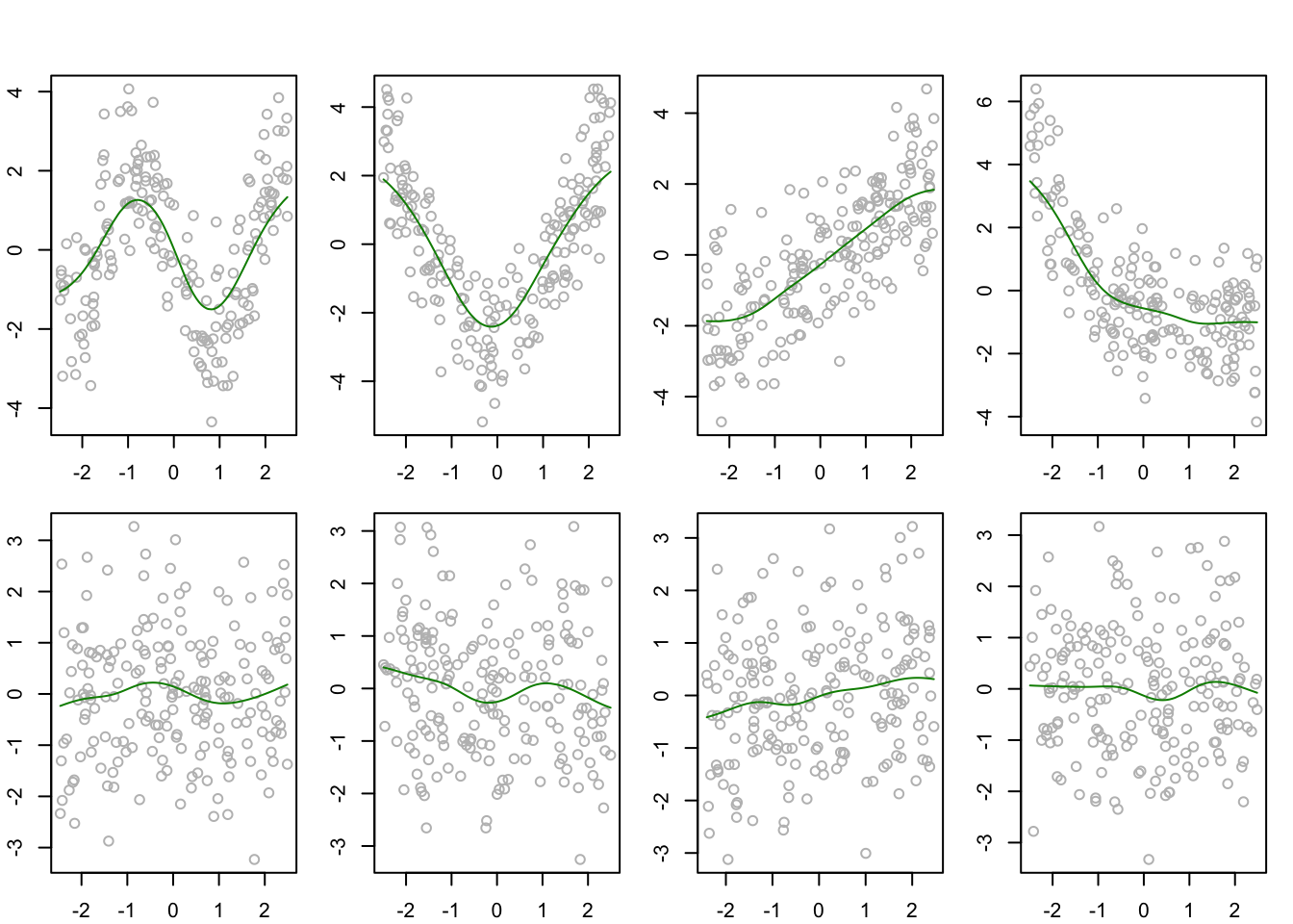
h <-0.5Snw <-array(0,dim=c(n,n,p)) # store smoother matrices in an arrayfor(j in1:p){ Sj <-dnorm(outer(X[,j],X[,j],"-")/h) Sj <- Sj /apply(Sj,2,sum) Snw[,,j] <- Sj}# center the response and obtain the backfitting estimatesYcent <- Y -mean(Y)M <-backfit(Ycent,Snw)par(mfrow =c(2,4), mar =c(2.1,2.1,1.1,1.1),oma =c(0,0,2,0))for(j in1:p){ Yj <- Ycent -apply(M[,-j],1,sum)plot(Yj ~ X[,j],col ="gray")lines(M[order(X[,j]),j]~sort(X[,j]), col =rgb(0,0.545,0))}
Backfitting estimators of additive components using Nadaraya-Watson smoothers
Note that the backfitting algorithm only returns the values of the estimated additive components at the design points, that is at the observed values of the predictors.
In order to evaluate an estimated additive component \(\hat m_j\) at a value \(x\) which is not a design point, one can re-apply the univariate smoother corresponding to the smoother matrix \(\mathbf{S}_j\) to the data points \((x_{1j},\hat Y_{1j}),\dots,(x_{nj},\hat Y_{nj})\), where \(\hat Y_{1j},\dots,\hat Y_{nj}\) are the entries of the vector \(\mathbf{Y}- \sum_{k\neq j}\hat{\mathbf{m}}_k\).
Note that one may construct the smoother matrix differently for each \(j\). For example, in the case of spline smoothing one might, for each predictor, position the knots at equally spaced quantiles of the observed values, resulting in a different set of knots for each \(j\).
Buja, Andreas, Trevor Hastie, and Robert Tibshirani. 1989. “Linear Smoothers and Additive Models.”The Annals of Statistics, 453–510.
Meier, Lukas, Sara Van de Geer, Peter Bühlmann, et al. 2009. “High-Dimensional Additive Modeling.”The Annals of Statistics 37 (6B): 3779–3821.