12  Bandwidth selection for the local polynomial estimator via crossvalidation

$$

$$

Here we will consider bandwidth selection via crossvalidation for the local polynomial estimator, of which the Nadaraya-Watson estimator is a special case.

This approach chooses the bandwidth \(h\) which minimizes the crossvalidation estimate of the mean squared error of prediction. For \(h > 0\) and some polynomial order \(k \geq 0\), set \[ \operatorname{CV}(h) = \frac{1}{n}\sum_{i=1}^n[Y_i - \hat m_{n,h,-i}^{\operatorname{LP}(k)}(x_i)]^2, \] where, for each \(i=1,\dots,n\), we define \(\hat m_{n,h,-i}^{\operatorname{LP}(k)}(x_i)\) as the local polynomial estimator computed after removing the pair \((x_i,Y_i)\) from the data and then evaluated at \(x_i\).

Lemma 12.1 (Crossvalidation for local polynomial estimators) Given weights \(W_{ni}(x)\), \(i=1,\dots,n\), such that the local polynomial estimator is given by \(\hat m_{n,h}^{\operatorname{LP}(k)} = \sum_{i=1}^n W_{ni}(x)Y_i\) for all \(x\), we have \[ \frac{1}{n}\sum_{i=1}^n[Y_i - \hat m_{n,h,-i}^{\operatorname{LP}(k)}(x_i)]^2 = \frac{1}{n}\sum_{i=1}^n\Big[\frac{Y_i - \hat m_{n,h}^{\operatorname{LP}(k)}(x_i)}{1-W_{ni}(x_i)}\Big]^2. \]

The above result allows one to compute the crossvalidation criterion \(\operatorname{CV}(h)\) without actually removing the data pairs \((x_i,Y_i)\), \(i=1,\dots,n\), one by one. It is only necessary to obtain the values of the local polynomial estimator, computed on the complete data set, at each design point \(x_1,\dots,x_n\). Then one can make a simple calculation involving the weights \(W_{ni}(x)\). Crossvalidation is therefore not costly in terms of computation time.

It is fairly simple to prove Lemma 12.1 in the case of the Nadaraya-Watson estimator (\(k=0\)), and this is left as an exercise. For \(k > 1\), the result is not as easy to establish; it is claimed on page 69 of Wasserman (2006).

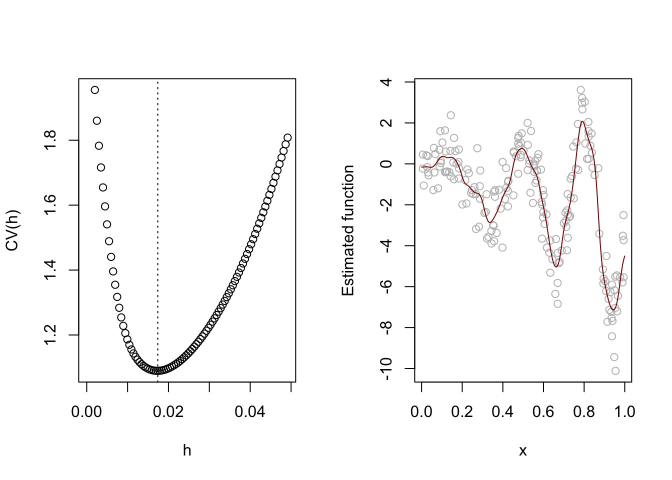
Figure 12.1 exhibits bandwidth selection via crossvalidation for the Nadaraya-Watson estimator.

# NW estimator
mNW <- function(x,data,K,h){
  
  Wx <- K((data$X - x)/h) / sum(K((data$X - x)/h))
  mNWx <- sum(Wx*data$Y)
  return(mNWx)

}

# choose h for NW estimator via crossvalidation
mNWcv <- function(data,K,nh = 100){
  
  # choose a sequence of candidate bandwidths
  dx <- diff(sort(data$X))
  hmin <- min(dx)
  hmax <- 2*max(dx)
  hh <- seq(hmin,hmax,length=nh)
  
  # compute CV criterion for each bandwidth
  CV <- numeric(nh)
  for(j in 1:nh){
    
    WW <- K( outer(data$X,data$X,FUN="-")/hh[j])
    WW <- (1/apply(WW,1,sum)) * WW
    mX <- WW %*% data$Y
    WX <- diag(WW)
    
    CV[j] <- mean(((data$Y - mX)/(1 - WX))^2)
    
  }
  
  # select bandwidth minimizing the CV criterion
  hcv <- hh[which.min(CV)]
  
  output <- list(CV = CV,
                 hh = hh,
                 hcv = hcv)
  
  return(output)

}


# true function m
m <- function(x) 5*x*sin(2*pi*(1 + x)^2) - (5/2)*x

# generate data
n <- 200
X <- runif(n)
e <- rnorm(n)
Y <- m(X) + e
data <- list(X = X,Y = Y)

mNWcv_out <- mNWcv(data,K = dnorm)

x <- seq(0,1,length=200)
mNW <- sapply(x,FUN = "mNW", data = data, K = dnorm, h = mNWcv_out$hcv)

par(mfrow = c(1,2))

plot(mNWcv_out$CV ~ mNWcv_out$hh,
     xlab = "h",
     ylab = "CV(h)")
abline(v = mNWcv_out$hcv, lty = 3)

plot(Y~X, col = "gray",
     xlab = "x",
     ylab = "Estimated function")
lines(mNW ~ x, col = rgb(0.545,0,0,1))

Figure 12.1: Bandwidth selection for the Nadaraya-Watson estimator on a synthetic data set.

Wasserman, Larry. 2006. All of Nonparametric Statistics. Springer Science & Business Media.