Definition 19.1 (Sparse additive model) The sparse additive model for observed data \((\mathbf{x}_1,Y_1),\dots,(\mathbf{x}_n,Y_n) \in [0,1]^p \times \mathbb{R}\) is \[
Y_i = m_1(x_{i1}) + \dots + m_p(x_{ip}) + \varepsilon_i,
\tag{19.1}\] for \(i = 1,\dots,n\), where \(m_1,\dots,m_p\) are unknown functions on \([0,1]\), \(\varepsilon_1,\dots,\varepsilon_n\) are independent random variables with mean \(0\) and variance \(\sigma^2\), and the set \[
\mathcal{A}= \{j : m_j \neq 0\}
\] has cardinality \(s < p\).
By \(m_j\neq 0\) we mean that \(m_j\) is not the zero function on \([0,1]\). Note that we have omitted the mean \(\mu\) in the sparse additive model definition, as we will center the \(Y_i\) to have mean zero and assume the identiability condition in Equation 16.2.
The sparse additive model assumes that some of the functions are the zero function, so that some of the covariates do not have any influence on the response.
Many estimators have been proposed in this setting. Such estimators typically aim to:
Identify which functions are nonzero.
Estimate these functions.
The idea is that if some functions can be identified as the zero function, we do not need to bother estimating them. So we don’t need to “use up” our data estimating every single one of the \(p\) unknown functions; rather, we can use our data to estimate a smaller number \(s\) of unknown functions (though we do “spend” some of our data trying to guess which functions are zero and which are not).
Of the myriad estimators we could discuss, we select one: the sparse backfitting estimator of Ravikumar et al. (2009).
Definition 19.2 (Soft-thresholded backfitting algorithm) Initialize \(\hat{\mathbf{m}}_1,\dots,\hat{\mathbf{m}}_p = \mathbf{0}\). Then for some \(\lambda > 0\) do: For \(j =1,\dots,p\) update \(\hat{\mathbf{m}}_j\) as
The norm \(\|\hat{\mathbf{m}}_j\|_n\) appearing in the algorithm is defined by \(\|\hat{\mathbf{m}}_j\|^2_n = n^{-1}\sum_{i=1}^n \hat m_j^2(x_{ij})\) for each \(j=1,\dots,p\). If this norm is small, the estimator is set to zero; if it is large, the estimator is shrunk towards zero.
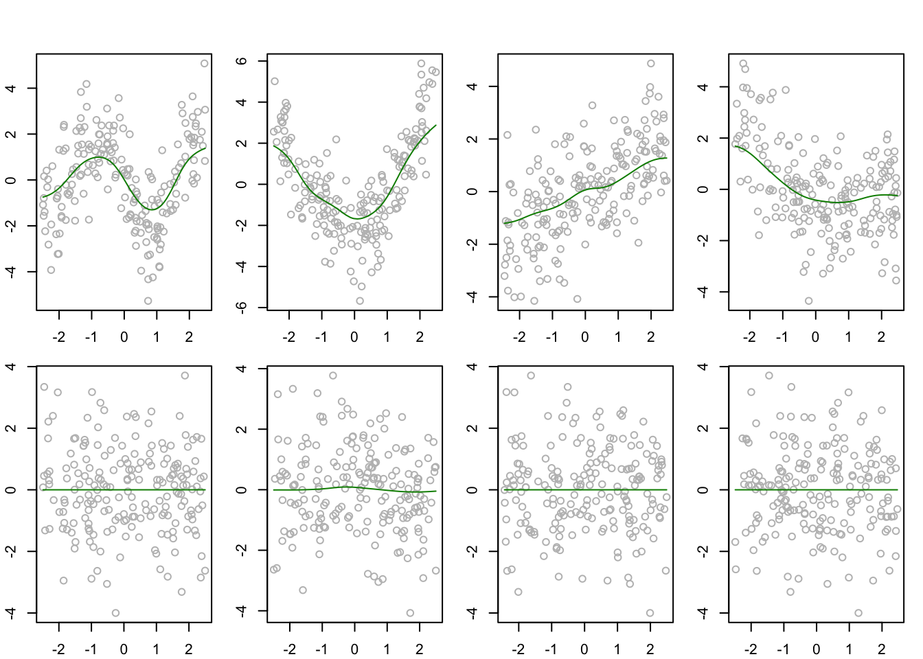
Figure 19.1 shows that the sparse backfitting estimator can result in additive component estimates which are the zero function.
Code
# generate datap <-8rho <-0.5n <-200m1 <-function(x){-2*sin(x*2)}m2 <-function(x){x^2-25/12}m3 <-function(x){x}m4 <-function(x){(exp(-x)-2/5*sinh(5/2))/2}# generate covariates marginally uniform and having correlation matrix RR <- rho^abs( outer(1:p,1:p,"-"))P <-2*sin( R * pi /6)X <- (pnorm( matrix(rnorm(n*p),ncol = p) %*%chol(P)) - .5) *5# make the true functions satisfy the identifiability conditionm1X <-m1(X[,1]) -mean(m1(X[,1]))m2X <-m2(X[,2]) -mean(m2(X[,2]))m3X <-m3(X[,3]) -mean(m3(X[,3]))m4X <-m4(X[,4]) -mean(m4(X[,4]))mu <-4Y <- mu + m1X + m2X + m3X + m4X +rnorm(n,0,1)# define backfitting functionspbackfit <-function(Y,S,lam,tol=1e-6){ n <-length(Y) p <-dim(S)[3] conv <-FALSE M <-matrix(0,n,p)while(conv ==FALSE){ M0 <- Mfor(j in1:p){ M[,j] <- S[,,j] %*% (Y -apply(M[,-j],1,sum))# soft-thresholding step mjn <-sqrt(mean(M[,j]^2))if(mjn >= lam){ M[,j] <- M[,j] * (mjn - lam) / mjn } else { M[,j] <-0 } M[,j] <- M[,j] -mean(M[,j]) } conv <-max(abs(M - M0)) < tol }return(M)}h <-0.4Snw <-array(0,dim=c(n,n,p)) # store smoother matrices in an arrayfor(j in1:p){ Sj <-dnorm(outer(X[,j],X[,j],"-")/h) Sj <- Sj /apply(Sj,2,sum) Snw[,,j] <- Sj}# center the response and obtain the sparse backfitting estimatesYcent <- Y -mean(Y)lam <- .25M <-spbackfit(Ycent,Snw,lam)par(mfrow =c(2,4), mar =c(2.1,2.1,1.1,1.1),oma =c(0,0,2,0))for(j in1:p){ Yj <- Ycent -apply(M[,-j],1,sum)plot(Yj ~ X[,j],col ="gray")lines(M[order(X[,j]),j]~sort(X[,j]), col =rgb(0,0.545,0))}
Figure 19.1: Sparse backfitting estimators of additive components using Nadaraya-Watson smoothers
Ravikumar, Pradeep, John Lafferty, Han Liu, and Larry Wasserman. 2009. “Sparse Additive Models.”Journal of the Royal Statistical Society: Series B (Statistical Methodology) 71 (5): 1009–30.