17  Bootstrap for the studentized sample mean

$$

$$

As before, assume throughout that \(X_1,\dots,X_n\) are independent, identically distributed random variables with mean \(\mu\) and variance \(\sigma^2 < \infty\). In this section, instead of considering the quantity \(Y_n = \sqrt{n}(\bar X_n - \mu)\), which is asymptotically distributed as \(\mathcal{N}(0,\sigma^2)\) as \(n \to \infty\), we will consider a studentized version \(T_{n} = \sqrt{n}(\bar X_n - \mu)/S_n\), which is asymptotically distributed as \(\mathcal{N}(0,1)\) as \(n \to \infty\) (\(S_n\) is the sample standard deviation). We will find that beginning with a studentized statistic can lead to better performance of bootstrap confidence intervals.

Let \(\bar X_n = n^{-1}\sum_{i=1}^n X_i\) and \(S_n^2 = (n-1)^{-1}\sum_{i=1}^n(X_i - \bar X_n)^2\) and consider the quantity \[ T_{n} \equiv \sqrt{n}(\bar X_n - \mu)/S_n\overset{\text{d}}{\longrightarrow}\mathcal{N}(0,1), \] where the convergence in distribution follows from the central limit theorem together with Slutzky’s theorem under the assumption \(\mathbb{E}|X_1|^3 <\infty\).

Note that the asymptotic distribution of \(T_n\) does not depend on any unknown parameters. Such a quantity that is a function of the data as well as some parameters and which has a known asymptotic distribution is called an asymptotic pivotal quantity. The bootstrap really shines when it is used to estimate the sampling distributions of pivotal quantities.

Now, for each \(n\geq 1\), define the cumulative distribution function \(G_{T_n}\) as \[ G_{T_n}(x) = \mathbb{P}(T_n \leq x) \] for all \(x \in \mathbb{R}\) and denote the corresponding quantile function by \(G^{-1}_{T_n}\). We observe, as before, that if one knew the function \(G^{-1}_{T_n}\), one could construct a confidence interval for \(\mu\) having coverage probability exactly equal to \(1-\alpha\) as

\[ \big[\bar X_n - G_{T_n}^{-1}(1-\alpha/2)S_n/\sqrt{n}, \bar X_n - G_{T_n}^{-1}(\alpha/2)S_n/\sqrt{n}\big]. \]

However, since the distribution \(G_{T_n}\) is unknown, we will have to replace the quantiles \(G_{T_n}^{-1}(1-\alpha/2)\) and \(G_{T_n}^{-1}(\alpha/2)\) with estimates. Below we define the bootstrap estimator of \(G_{T_n}\).

Definition 17.1 (Bootstrap estimator of \(G_{T_n}\)) Conditional on \(X_1,\dots,X_n\), introduce random variables \(X_1^*,\dots,X_n^*\) such that \(X_1^*,\dots,X_n^*|X_1,\dots,X_n \overset{\text{ind}}{\sim}\hat F_n\), where \(\hat F_n\) is the empirical distribution of \(X_1,\dots,X_n\), and define the bootstrap version \(T_n^*\) of \(T_n =\sqrt{n}(\bar X_n - \mu)/S_n\) as \[ T_n^* \equiv \sqrt{n}(\bar X_n^* - \bar X_n)/S_n^*, \] where \(\bar X_n^* = n^{-1}\sum_{i=1}^n X_i\) and \((S_n^*)^2 = (n-1)^{-1}\sum_{i=1}^n(X_i^* - \bar X_n^*)^2\). Then the bootstrap estimator \(\hat G_{T_n}\) of \(G_{T_n}\) is defined as \[ \hat G_{T_n}(x) = \mathbb{P}(T_n^* \leq x | X_1,\dots,X_n) \] for all \(x \in \mathbb{R}\).

Once one obtains the bootstrap estimate \(\hat G_{T_n}(x)\) for all \(x \in \mathbb{R}\), one can construct the bootstrap confidence interval \[ \big[\bar X_n - \hat G_{T_n}^{-1}(1-\alpha/2)S_n/\sqrt{n}, \bar X_n - \hat G_{T_n}^{-1}(\alpha/2)S_n/\sqrt{n}\big]. \]

Because it is prohibitively computationally expensive to compute the bootstrap estimator \(\hat G_{T_n}(x)\) of \(G_{T_n}(x)\) exactly, we turn, as before, to Monte Carlo simulation:

Definition 17.2 (Monte Carlo approximation to bootstrap estimator \(\hat G_{T_n}\)) Choose a large \(B\). Then for \(b=1,\dots,B\) do:

• Draw \(X_1^{*(b)},\dots,X_n^{*(b)}\) with replacement from \(X_1,\dots,X_n\).
• Compute \(T_n^{*(b)} =\sqrt{n}(\bar X_n^{*(b)} - \bar X_n)/S_n^{*(b)}\), where \(\bar X^{*(b)} = n^{-1}\sum_{i=1}^n X_i^{*(b)}\) and \((S_n^{*(b)})^2 = (n-1)^{-1}\sum_{i=1}^n(X_i^{*(b)} - \bar X_n^{*(b)})^2\).

Then set \(\hat G_{T_n}(x) = B^{-1}\sum_{b=1}^B \mathbf{1}(T_n^{*(b)} \leq x)\) for all \(x \in \mathbb{R}\).

Monte Carlo approximations to the quantiles \(\hat G^{-1}_{T_n}(u)\) for \(u \in (0,1)\) may be obtained as follows: Sort the bootstrap realizations \(T_n^{*(b)}\) from the Monte Carlo simulation such that \(T_n^{*(1)} \leq \dots \leq T_n^{*(b)}\) and then set \[ \hat G^{-1}_{T_n}(u) = T_n^{*(\lceil u B\rceil)} \] for all \(u \in (0,1)\).

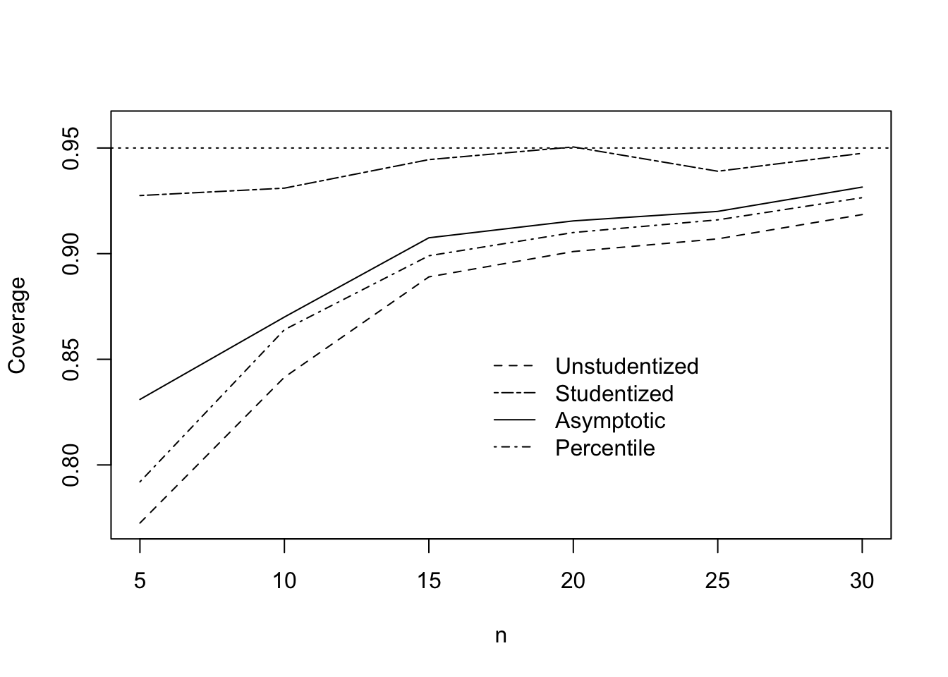
Figure 17.1 shows, over an increasing sample size \(n\), the realized coverage of \(95\%\) bootstrap intervals based on the pivots \(Y_n\) and \(T_n\) as well as of the interval \(\bar X_n \pm z_{\alpha/2}S_n/\sqrt{n}\) based on the asymptotic distribution of \(T_n\). Also included is the coverage performance of the percentile bootstrap interval discussed in Chapter 22.

alpha <- 0.05
nn <- seq(5,30,by=5)
B <- 500
S <- 2000
shape <- 1.5
scale <- 4
mu <- shape * scale
zval <- qnorm(1 - alpha/2)

Ycvg <- Yaw <- numeric(length(nn))
Tcvg <- Taw <- numeric(length(nn))
Zcvg <- Zaw <- numeric(length(nn))
Pcvg <- Paw <- numeric(length(nn))

for(j in 1:length(nn)){

  n <- nn[j]
  
  Ycov <- Yw <- numeric(S)
  Tcov <- Tw <- numeric(S)
  Zcov <- Zw <- numeric(S)
  Pcov <- Pw <- numeric(S)
  
  for(s in 1:S){

    X <- rgamma(n,shape = shape, scale = scale)
    Xbar <- mean(X)
    Sn <- sd(X)
    Xb <- matrix(X[sample(1:n,n*B,replace = TRUE)],n,B)
    Xbbar <- apply(Xb,2,mean)
    Snb <- apply(Xb,2,sd)

    Yb <- sqrt(n)*(Xbbar - Xbar)
    Yb_srt <- sort(Yb)

    Ylo <- Xbar - Yb_srt[ceiling((1-alpha/2)*B)] / sqrt(n)
    Yup <- Xbar - Yb_srt[ceiling(alpha/2*B)] / sqrt(n)
    Ycov[s] <- (Ylo < mu) & (Yup > mu)
    Yw[s] <- Yup - Ylo
    
    Tb <- sqrt(n)*(Xbbar - Xbar) / Snb
    Tb_srt <- sort(Tb)

    Tlo <- Xbar - Tb_srt[ceiling((1-alpha/2)*B)] * Sn / sqrt(n)
    Tup <- Xbar - Tb_srt[ceiling(alpha/2*B)] * Sn / sqrt(n)
    Tcov[s] <- (Tlo < mu) & (Tup > mu)
    Tw[s] <- Tup - Tlo

    Zlo <- Xbar - zval * Sn / sqrt(n)
    Zup <- Xbar + zval * Sn / sqrt(n)
    Zcov[s] <- (Zlo < mu) & (Zup > mu)
    Zw[s] <- Zup - Zlo
    
    Xbbar_srt <- sort(Xbbar)
    Plo <- Xbbar_srt[ceiling(alpha/2*B)]
    Pup <- Xbbar_srt[ceiling((1-alpha/2)*B)]
    Pcov[s] <- (Plo < mu) & (Pup > mu)
    Pw[s] <- Pup - Plo

  }

  Ycvg[j] <- mean(Ycov)
  Yaw[j] <- mean(Yw)
  
  Tcvg[j] <- mean(Tcov)
  Taw[j] <- mean(Tw)
  
  Zcvg[j] <- mean(Zcov)
  Zaw[j] <- mean(Zw)
  
  Pcvg[j] <- mean(Pcov)
  Paw[j] <- mean(Pw)
  
}

plot(NA,
     ylim = range(Ycvg,Tcvg,Zcvg,Pcvg,.96),
     xlim = range(nn),
     xlab = "n",
     ylab = "Coverage")

lines(Ycvg ~ nn, lty = 2)
lines(Tcvg ~ nn, lty = 6)
lines(Zcvg ~ nn, lty = 1)
lines(Pcvg ~ nn, lty = 4)
abline( h = 1 - alpha, lty = 3)

x.pos <- grconvertX(x = .5, from ="nfc", to = "user")
y.pos <- grconvertY(y = .5, from ="nfc", to = "user")
legend(x = x.pos,
       y = y.pos,
       legend = c("Unstudentized",
                  "Studentized",
                  "Asymptotic",
                  "Percentile"),
       lty = c(2,6,1,4),
       bty = "n")

Figure 17.1: Coverage of \(95\%\) bootstrap intervals over increasing \(n\) based on \(Y_n\) (unstudentized) and \(T_n\) (studentized) as well as of the interval based on the asymptotic distribution of \(T_n\) and the percentile bootstrap interval when \(X_1,\dots,X_n\) have the Gamma distribution with mean \(6\) and variance \(24\).

We note that the interval based on \(T_n\), which we may call the “studentized” bootstrap interval, achieves coverage closer to the nominal level of \(95\%\) at much smaller sample sizes than the asymptotic interval and the bootstrap interval based on \(Y_n\), which we may call the “unstudentized” bootstrap interval.

Having taken a glimpse at the numerical performance of the bootstrap confidence intervals based on \(Y_n\) and \(T_n\), we will study whence the superior performance of the \(T_n\)-based interval comes.