Suppose we observe data \((\mathbf{x}_1,Y_1),\dots,(\mathbf{x}_n,Y_n)\in [0,1]^p\times \mathbb{R}\), where \[
Y_i = m(\mathbf{x}_i) + \varepsilon_i,
\]\(i = 1,\dots,n\), where \(m\) is an unknown function on \([0,1]^p\) and \(\varepsilon_1,\dots,\varepsilon_n\) are independent random variables with mean \(0\) and variance \(\sigma^2\).
As before, we will most of the time treat \(\mathbf{x}_1,\dots,\mathbf{x}_n\) as deterministic (fixed).
Our goal will be to estimate the unknown function \(m\).
Definition 15.1 (Multivariate Nadaraya-Watson estimator) A multivariate version of the Nadaraya-Watson estimator is given by \[
\hat m_{n}^{\text{NW}}(\mathbf{x}) = \frac{\sum_{i=1}^n Y_i K(h^{-1}(\mathbf{x}_i - \mathbf{x}))}{\sum_{i'=1}^nK(h^{-1}(\mathbf{x}_{i'} - \mathbf{x}))}
\] for all \(\mathbf{x}\in [0,1]^p\) for some kernel function \(K:\mathbb{R}^p \to \mathbb{R}\) and bandwidth \(h > 0\).
The kernel is often of the form \(K(\mathbf{u}) = \prod_{j=1}^p G(u_j)\) where \(G\) a univariate kernel like \[
G(z) = \phi(z) \quad \text{ or } \quad G(z) = \frac{3}{4}(1 - z^2)\mathbf{1}(|z| \leq 1).
\]
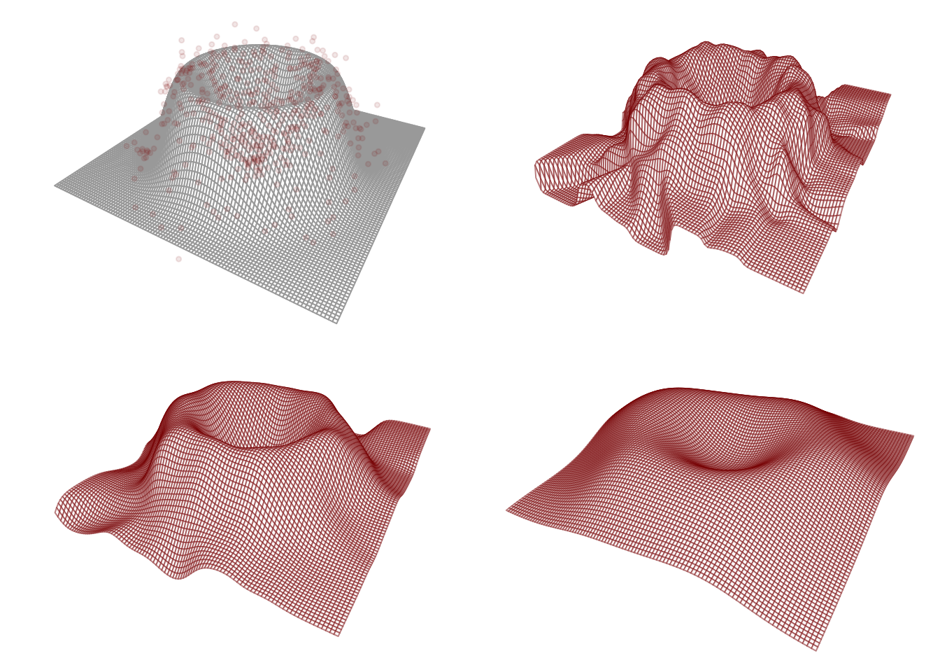
Here is an example of what the estimator \(\hat m_{n}^{\text{NW}}(\mathbf{x})\) can look like when \(p=2\).
Code
m <-function(x){ u <-sqrt(sum(x^2)) val1 <-32/3* u^3* ( ( (0<= u) & ( u <1/4))) val2 <- (32* u^2-32* u^3-8* u +2/3 ) * ( (1/4<= u) & ( u <2/4) ) val3 <- (32* ( 1- u )^2-32* ( 1- u )^3-8* ( 1- u ) +2/3) * ( (2/4<= u) & ( u <3/4) ) val4 <-32/3* ( 1- u )^3* ( (3/4<= u) & ( u <1)) val <- val1 + val2 + val3 + val4return(val)}n <-500X <-matrix(0,n,2)theta <-runif(n,0,2*pi)r <-rbeta(n,2,2)X[,1] <- r*cos(theta)X[,2] <- r*sin(theta)Y <-apply(X,1,m) +rnorm(n,0,.1)Ker <- dnormbivNW <-function(x, data =list(X,Y), K, h){ X <- data$X Y <- data$Y num <-sum(Y *K((X[,1] - x[1] )/h) *K((X[,2] - x[2])/h)) den <-sum( K((X[,1] - x[1] )/h) *K((X[,2] - x[2])/h)) val <- num / denreturn(val)}grid <-100x1 <- x2 <-seq(-1,1,length=grid)hh <-c(0.05,0.1,0.2)mx <-matrix(0,grid,grid) mNWx <-array(0,dim =c(grid,grid,length(hh)))for(i in1:grid)for( j in1:grid){ mx[i,j] <-m(c(x1[i],x2[j]))for(k in1:length(hh)){ mNWx[i,j,k] <-bivNW(c(x1[i],x2[j]),data =list(X = X, Y = Y), K = dnorm, h = hh[k]) } }par(mfrow=c(2,2), mar=c(0,0,0,0))persp_out <-persp(x = x1,y = x2,z = mx,theta =30,phi =30,r =sqrt(1),d =1,box =FALSE,scale =FALSE,border ="dark gray")points(trans3d(x = X[,1], y = X[,2], z = Y, pmat = persp_out),pch =19,cex = .6,col =rgb(.545,0,0,.1))for(k in1:length(hh)){ persp_out <-persp(x = x1,y = x2,z = mNWx[,,k],theta =30,phi =30,r =sqrt(1),d =1,box =FALSE,scale =FALSE,border =rgb(.545,0,0,.5))}
Figure 15.1: Nadaraya-Watson estimator in \(p=2\) setting at three bandwidth choices. Top left shows the true function \(m\).
The following is a result about the variance \(\mathbb{V}\hat m_n^{\text{NW}}(\mathbf{x})\).
Proposition 15.1 (Bounds on the variance of the multivariate Nadaraya-Watson estimator) Given a kernel function \(K\) and a bandwidth \(h\), suppose \(\mathbf{x}_1,\dots,\mathbf{x}_n \in [0,1]^p\) are deterministic such that for some \(n_0>0\) we have \[
0 < c_1 \leq \frac{1}{nh^p}\sum_{i=1}^n K(h^{-1}(\mathbf{x}_i - \mathbf{x})) \leq c_1^{-1}
\] and \[
0 < c_2 \leq \frac{1}{nh^p}\sum_{i=1}^n K^2(h^{-1}(\mathbf{x}_i - \mathbf{x})) \leq c_2^{-1}
\] for some \(c_1,c_2 > 0\) for all \(x \in [0,1]^p\) for all \(n \geq n_0\). Then for all \(n \geq n_0\), we have \[
\frac{\sigma^2}{nh^p} c_1^2 c_2 \leq \mathbb{V}\hat m_n^{\text{NW}}(\mathbf{x}) \leq \frac{\sigma^2}{nh^p} \frac{1}{c_1^2 c_2}
\tag{15.1}\]
for all \(\mathbf{x}\in [0,1]^p\).
Just as in the case of multivariate kernel density estimation, we encounter the curse of dimensionality. That is, the dimension \(p\) appears in our bounds for the variance just as in the case of multivariate kernel density estimation.
Write \(\hat m_n^\text{NW}(\mathbf{x}) = \sum_{i=1}^n W_{ni}(\mathbf{x})Y_i\) with \[
W_{ni}(\mathbf{x}) = \frac{K(h^{-1}(\mathbf{x}_i - \mathbf{x}))}{\sum_{i'=1}^nK(h^{-1}(\mathbf{x}_{i'} - \mathbf{x}))}.
\] Then for all \(n \geq n_0\) we have \[\begin{align}
\mathbb{V}\hat m_n^{\text{NW}}(\mathbf{x}) &= \sum_{i=1}^n W^2_{ni}(\mathbf{x}) \sigma^2 \\
&= \sigma^2 \sum_{i=1}^n \frac{K^2(h^{-1}(\mathbf{x}_i - \mathbf{x}))}{[\sum_{i'=1}^nK(h^{-1}(\mathbf{x}_{i'} - \mathbf{x}))]^2} \\
&= \frac{\sigma^2}{nh^p}\frac{(nh^p)^{-1}\sum_{i=1}^n K^2(h^{-1}(\mathbf{x}_i - \mathbf{x}))}{[(nh^p)^{-1}\sum_{i'=1}^n K(h^{-1}(\mathbf{x}_{i'} - \mathbf{x}))]^2}
\end{align}\] The result follows from applying the bounds in (Equation 15.1).
In order to analyze the bias, one would need, just as in the case of multivariate kernel density estimation, to make an assumption about the smoothness of the unknown function \(m\). If one, for example, places \(m\) in a \(p\)-dimensional Hölder class \(\mathcal{H}_p(\beta,L)\) and chooses a \(p\)-dimensional kernel \(K\) of corresponding order, one could bound the magnitude of the bias by a constant times \(h^{\beta}\). We omit the details.
One way to mitigate the curse of dimensionality is to make assumptions about \(m\) which place it in a smaller class of functions. An assumption known as additivity is very often used.