41Bootstrap confidence bands in nonparametric regression
$$
$$
We now consider using the bootstrap to produce confidence bands for the function \(m\) in the nonparametric regression model in Definition 40.1. We consider, as in the previous section, the constant-variance case as well as the non-constant-variance case.
First consider the case \(\sigma_1^2 = \dots = \sigma_n^2 = \sigma^2\), under which the relevant pivotal quantity for a constructing confidence band is \[
T_n = \sup_{x\in[0,1]} \left|\frac{\hat m_n(x) - \mathbb{E}\hat m_n(x)}{\hat \sigma_n \sqrt{\sum_{i=1}^n W^2_{ni}(x)}}\right|,
\] as discussed in the previous section. Define the cumulative distribution function of \(T_n\) as \[
G_{T_n}(x) = \mathbb{P}(T_n \leq x), \quad x \in \mathbb{R},
\] and the corresponding quantile function as \(G_{T_n}^{-1}\). Now, if \(G_{T_n}\) were known, an asymptotic \((1-\alpha)100\%\) confidence band for the function \(m(x)\) over \(x \in [0,1]\) could be constructed as the collection of intervals \[
\textstyle I_{T_n}(x) = \Big[\hat m_n(x) \pm G_{T_n}^{-1}(1-\alpha) \hat \sigma_n \sqrt{\sum_{i=1}^n W^2_{ni}(x)}\Big], \quad x \in [0,1].
\] The reason the coverage is only asymptotically \(1-\alpha\) instead of exactly \(1-\alpha\) is due to the the use of the centering \(\mathbb{E}\hat m_n(x)\) instead of \(m(x)\) in the definition of \(T_n\), but we will proceed under the assumption that the difference between these—the bias—becomes asymptotically negligible.
We define a bootstrap estimator of \(G_{T_n}\) as follows:
Definition 41.1 (Residual bootstrap estimator of \(G_{T_n}\)) Conditional on \(Y_1,\dots,Y_n\), introduce independent random variables \(\varepsilon_1^*,\dots,\varepsilon_n^*\) distributed according to the empirical distribution of the residuals \(\hat\varepsilon_i = Y_i - \hat m_n(x_i)\), \(i=1,\dots,n\). Then set \(Y_i^* = \hat m_n(x_i) + \varepsilon_i^*\) for \(i=1,\dots,n\) and for each \(x \in [0,1]\) set \(\hat m_n^*(x) = \sum_{i=1}^nW_{ni}(x)Y_i^*\). Then construct \(\hat \sigma_n^*\) as in Equation 40.3 based on \((x_1,Y_1^*),\dots,(x_n,Y_n^*)\) and set \[
T_n^* = \sup_{x\in[0,1]} \left|\frac{\hat m_n^*(x) - \mathbb{E}_* \hat m_n^*(x)}{\hat \sigma_n^* \sqrt{\sum_{i=1}^n W^2_{ni}(x)}}\right|,
\] noting that \(\hat m_n^*(x) - \mathbb{E}_* \hat m_n^*(x) = \sum_{i=1}^nW_{ni}(x)\varepsilon_i^*\) for each \(x \in[0,1]\). Then the residual bootstrap estimator of \(G_{T_n}\) is defined as \[
\hat G_{T_n}(x) = \mathbb{P}_*(T^*_n \leq x), \quad x \in \mathbb{R}.
\]
Having obtained the residual bootstrap estimator of \(\hat G_{T_n}\) and the corresponding quantile function \(\hat G_{T_n}^{-1}\), the residual bootstrap confidence band for \(m(x)\) over \(x \in [0,1]\) is constructed as the set of intervals \[
\textstyle \hat I_{T_n}(x) = \Big[\hat m_n(x) \pm \hat G_{T_n}^{-1}(1 - \alpha) \hat \sigma_n \sqrt{\sum_{i=1}^n W^2_{ni}(x)}\Big], \quad x \in [0,1].
\tag{41.1}\] To obtain a Monte Carlo approximation to the set of intervals \(\hat I_{T_n}(x)\), \(x \in [0,1]\), one may generate independent realizations \(T_n^{*(1)},\dots,T_n^{*(B)}\) for some large \(B\), where for each \(b = 1,\dots,B\) we set \[
T_n^{*(b)} = \max_{j \in \{0,\dots,N\}} \left|\frac{\hat m_n^*(j/N) - \mathbb{E}_* \hat m_n^*(j/N)}{\hat \sigma_n^* \sqrt{\sum_{i=1}^n W^2_{ni}(j/N)}}\right|
\] for some large \(N\) in order to approximate the supremum. Then, after sorting the Monte Carlo realizations of \(T_n^*\) such that \(T_n^{*(1)}\leq\dots \leq T_n^{*(B)}\), we construct the bootstrap confidence band for \(m\) by replacing \(G_{T_n}^{-1}(1 - \alpha)\) in Equation 41.1 with \(T_n^{*(\lceil (1 - \alpha)B \rceil)}\).
In the case in which \(\sigma_1^2,\dots,\sigma_n^2\) may not all be equal, we consider the pivotal quantity \[
H_n = \sup_{x\in[0,1]} \left|\frac{\hat m_n(x) - \mathbb{E}\hat m_n(x)}{\sqrt{\sum_{i=1}^n W^2_{ni}(x)\hat \varepsilon_i^2}}\right|.
\] Letting \(G_{H_n}\) represent the cumulative distribution function of \(H_n\) and \(G_{H_n}^{-1}\) its quantile function, an approximate \((1 - \alpha)100\%\) confidence band is given by the set of intervals \[
I_{H_n}(x) = \Big[\hat m_n(x) \pm G_{H_n}^{-1}(1-\alpha) \sqrt{\sum_{i=1}^n W^2_{ni}(x)\hat \varepsilon_i^2}\Big], \quad x \in [0,1].
\] As in the constant-variance case, we will estimate \(G_{H_n}^{-1}(1-\alpha)\) with a bootstrap estimator.
Definition 41.2 (Residual bootstrap estimator of \(G_{T_n}\)) Conditional on \(Y_1,\dots,Y_n\) define the residuals \(\hat\varepsilon_i = Y_i - \hat m_n(x_i)\), \(i=1,\dots,n\), and introduce independent random variables \(\varepsilon_1^{*W},\dots,\varepsilon_n^{*W}\) distributed such that (i) \(\mathbb{E}_*[ \varepsilon_i^{*W}] = 0\), (ii) \(\mathbb{E}_*[ (\varepsilon_i^{*W})^2] = \hat \varepsilon_i^2\), and (iii) \(\mathbb{E}_*[ (\varepsilon_i^{*W})^3] = \hat \varepsilon_i^3\) for \(i=1,\dots,n\). Then set \(Y_i^{*W} = \hat m_n(x_i) + \varepsilon_i^{*W}\) for \(i=1,\dots,n\) and for each \(x \in [0,1]\) set \(\hat m_n^{*W}(x) = \sum_{i=1}^nW_{ni}(x)Y_i^{*W}\). Lastly, define \(\hat \varepsilon_i^{*W} = Y_i^{*W} - \hat m_n^{*W}(x_i)\) for \(i=1,\dots,n\) and set \[
H_n^{*W} = \sup_{x\in[0,1]} \left|\frac{\hat m_n^{*W}(x) - \mathbb{E}_* \hat m_n^{*W}(x)}{\sqrt{\sum_{i=1}^n W^2_{ni}(x)(\hat \varepsilon_i^{*W}})^2}\right|,
\] noting that \(\hat m_n^{*W}(x) - \mathbb{E}_* \hat m_n^{*W}(x) = \sum_{i=1}^nW_{ni}(x)\varepsilon_i^{*W}\) for each \(x \in[0,1]\). Then the wild bootstrap estimator of \(G_{H_n}\) is defined as \[
\hat G_{H_n}(x) = \mathbb{P}_*(H^{*W}_n \leq x), \quad x \in \mathbb{R}.
\]
The wild bootstrap \((1-\alpha)100\%\) confidence band for \(m\) over \(x \in [0,1]\) is then constructed as the collection of intervals \[
\textstyle I_{H_n}(x) = \Big[\hat m_n(x) \pm \hat G_{H_n}^{-1}(1-\alpha) \sqrt{\sum_{i=1}^n W^2_{ni}(x)\hat \varepsilon_i^2}\Big], \quad x \in [0,1].
\tag{41.2}\] As in the constant-variance case, one can replace \(\hat G_{H_n}^{-1}(1-\alpha)\) by a Monte Carlo approximation \(H_n^{*W(\lceil (1 - \alpha) B\rceil)}\), where this the \(1-\alpha\) quantile of the empirical distribution of some number \(B\) of Monte Carlo draws of \(H_n^{*W}\).
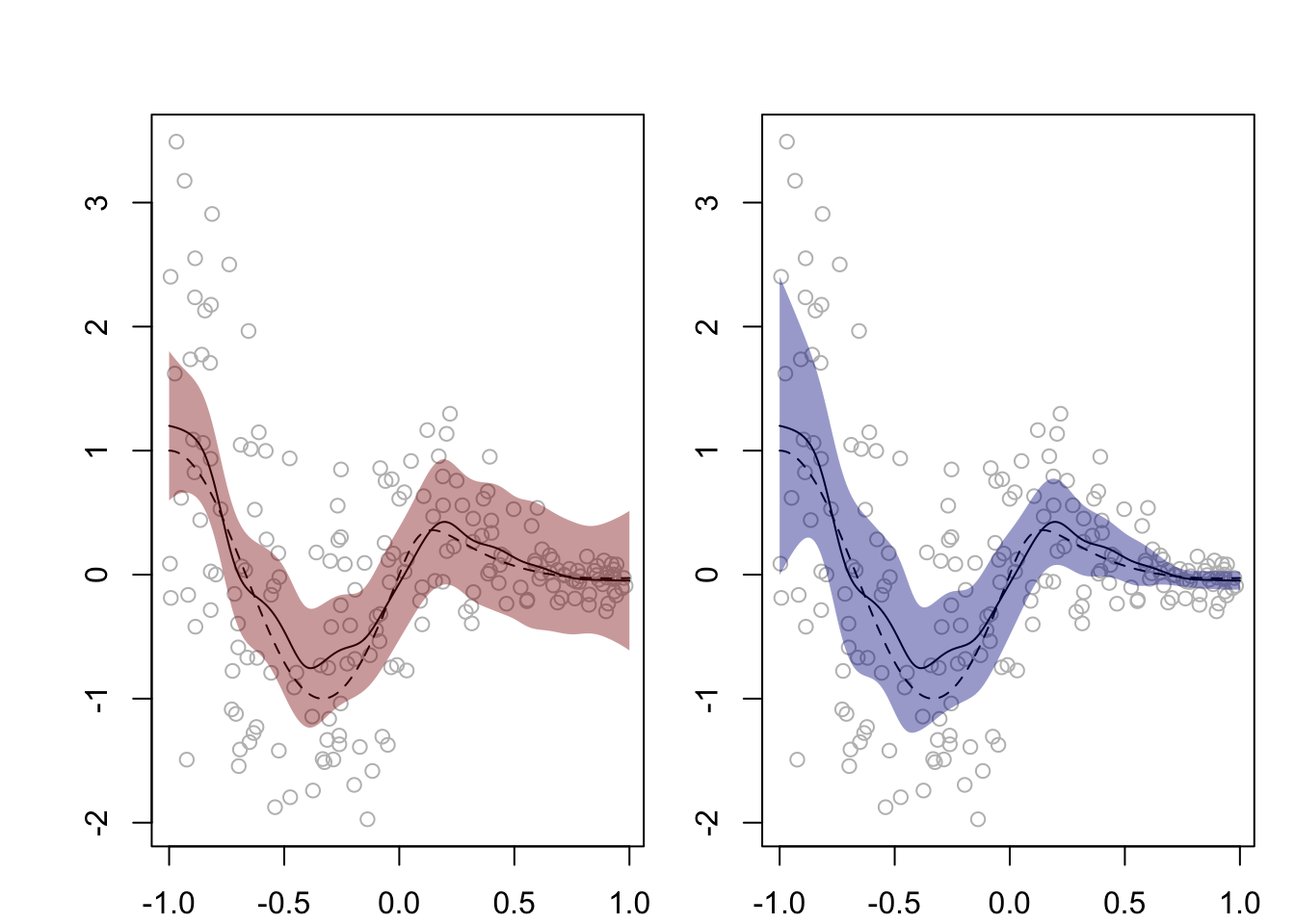
Figure 41.1 shows the residual bootstrap confidence band from Equation 41.1 and the wild bootstrap confidence band from Equation 41.2 on a single simulated data set. The bands are based on the Nadaraya-Watson estimator under the Gaussian kernel. The method of Das, Gregory, and Lahiri (2019) was used to generate the wild bootstrap error terms.
Code
# function for computing residual or wild bootstrap confidence bandsbootCBnw <-function(X,Y,h,alpha,xlims,het =FALSE,N=500,B=500){ n <-length(Y) x <-seq(xlims[1],xlims[2],length=N)# obtain function estimates at x Wx <-dnorm(outer(x,X,FUN="-"),0,h) Wx <- Wx /apply(Wx,1,sum) # scales each row mx_hat <-drop(Wx %*% Y)# obtain residuals S <-dnorm(outer(X,X,FUN="-"),0,h) S <- S /apply(S,1,sum) Yhat <-drop(S %*% Y) ehat <- Y - Yhatif(het == F){ ordX <-order(X) sigma_hat <-sqrt(sum(diff(Y[ordX])^2) / (2* (n -1))) Mx <- Wx /sqrt(apply(Wx^2,1,sum))# residual bootstrap Tn_boot <-numeric(B)for(b in1:B){ e_boot <- ehat[sample(c(1:n),n,replace=TRUE)] Y_boot <- Yhat + e_boot sigma_hat_boot <-sqrt(sum(diff(Y_boot[ordX])^2) / (2* (n -1))) Tn_boot[b] <-max(abs(Mx %*% e_boot) / sigma_hat_boot) } Ga <-sort(Tn_boot)[ceiling((1-alpha)*B)] me <- Ga * sigma_hat *sqrt(apply(Wx^2,1,sum)) lo <- mx_hat - me up <- mx_hat + me } elseif(het == T){# wild bootstrap Hn_boot <-numeric(B)for(b in1:B){ U_boot <-4*rbeta(n, shape1 =1/2, shape2 =3/2) -1 e_boot <- ehat * U_boot Y_boot <- Yhat + e_boot Yhat_boot <-drop(S %*% Y_boot) ehat_boot <- Y_boot - Yhat_boot Hn_boot[b] <-max(abs(Wx %*% e_boot /sqrt(Wx^2%*% ehat_boot^2))) } Ga <-sort(Hn_boot)[ceiling((1-alpha)*B)] me <- Ga *sqrt(Wx^2%*% ehat^2) lo <- mx_hat - me up <- mx_hat + me } output <-list(lo = lo,up = up,mx_hat = mx_hat,x = x)return(output)}# generate some datam <-function(x){sin(3* pi * x /2)/(1+18* x^2*(sign(x) +1))}n <-200X <-runif(n,-1,1)sigma <- (1.5- X)^2/4error <-rnorm(n,0,sigma)Y <-m(X) + error# now obtain the confidence bandsN <-300B <-500h <-0.08alpha <-0.05rbootCB <-bootCBnw(X,Y,h,alpha,xlims =c(-1,1),het = F,N = N)wbootCBhet <-bootCBnw(X,Y,h,alpha,xlims =c(-1,1),het = T, N=N)# make plotspar(mfrow=c(1,2),mar=c(2.1,2.1,1.1,1.1),oma =c(0,2,2,0))plot(Y~X,col="gray")lines(rbootCB$mx_hat ~ rbootCB$x)lines(m(rbootCB$x) ~ rbootCB$x, lty =2)polygon(x =c(rbootCB$x,rbootCB$x[N:1]),y =c(rbootCB$lo,rbootCB$up[N:1]), col =rgb(.545,0,0,.4),border =NA)plot(Y~X,col="gray")lines(wbootCBhet$mx_hat ~ wbootCBhet$x)lines(m(wbootCBhet$x) ~ wbootCBhet$x, lty =2)polygon(x =c(wbootCBhet$x,wbootCBhet$x[N:1]),y =c(wbootCBhet$lo,wbootCBhet$up[N:1]), col =rgb(0,0,.545,.4),border =NA)
Figure 41.1: Asymptotic 95% residual (left) and wild bootstrap (right) confidence bands from Equation 41.1 and Equation 41.2 based on the Nadaraya–Watson estimator (with the Gaussian kernel) for a nonparametric regression function assuming constant variance and allowing non-constant variance, respectively.
Das, Debraj, Karl Gregory, and Soumendra Lahiri. 2019. “Perturbation Bootstrap in Adaptive Lasso.”The Annals of Statistics 47 (4): 2080–2116.