5  Multivariate kernel density estimation

$$

$$

So far we have considered estimation of a univariate density. Now we will suppose we observe \(\mathbf{X}_1,\dots,\mathbf{X}_n \in \mathbb{R}^d\) with dimension \(d \geq 1\) which are independent realizations of a random vector \(\mathbf{X}\in \mathbb{R}^d\) having density \(f\) on \(\mathbb{R}^d\). For each \(i= 1,\dots,n\), index the entries in \(\mathbf{X}_i\) such that \(\mathbf{X}_i = (X_{i1},\dots,X_{id})^T\).

Given a \(d\)-dimensional kernel function \(K_d:\mathbb{R}^d \to \mathbb{R}\), consider the multivariate kernel density estimator (KDE) of \(f\) given by \[ \hat f_{n,\mathbf{H}}(\mathbf{x}) = \frac{1}{n|\mathbf{H}|^{1/2}}\sum_{i=1}^nK_d\Big(\mathbf{H}^{-1/2}(\mathbf{X}_i - \mathbf{x})\Big) \] for all \(\mathbf{x}\in \mathbb{R}^d\), where \(\mathbf{H}\) is a positive definite bandwidth matrix.

Proposition 5.1 (Validity of multivariate kernel density estimator) If \(K_d : \mathbb{R}^d\to \mathbb{R}\) is a density then \(\hat f_{n,\mathbf{H}}\) is a density.

Proof of Proposition 5.1

If \(K_d\) is a density then \(K_d(\mathbf{x}) \geq 0\) for all \(\mathbf{x}\in \mathbb{R}^d\) and \(\int_{\mathbb{R}^d}K_d(\mathbf{x})d\mathbf{x}= 1\). Therefore \(\hat f_{n,\mathbf{H}}(\mathbf{x}) \geq 0\) for all \(\mathbf{x}\in \mathbb{R}^d\) and \[\begin{align*} \int_{\mathbb{R}^d}\hat f_{n,\mathbf{H}}(\mathbf{x}) d\mathbf{x}&= \frac{1}{n}\sum_{i=1}^n\int_{\mathbb{R}^d}\frac{1}{|\mathbf{H}|^{1/2}}K_d\Big(\mathbf{H}^{-1/2}(\mathbf{X}_i - \mathbf{x})\Big) d\mathbf{x}\\ &= \frac{1}{n} \sum_{i=1}^n\int_{\mathbb{R}^d}K_d(\mathbf{u}_i)d\mathbf{u}_i\\ &= 1, \end{align*}\] using for each \(i=1,\dots,n\) the substitution \(\mathbf{u}_i = \mathbf{H}^{-1/2}(\mathbf{X}_i - \mathbf{x})\), for which the absolute value of the Jacobian is \(|\mathbf{H}|^{1/2}\). Therefore \(\hat f_{n,\mathbf{H}}\) is a density.

For further analysis, we will consider a simpler version of \(\hat f_{n,\mathbf{H}}\) corresponding to the choice \(\mathbf{H}= h^2 \mathbf{I}_d\) for some scalar bandwidth \(h > 0\). Define \[ \hat f_{n,h}(\mathbf{x}) = \frac{1}{nh^d}\sum_{i=1}^n K_d(h^{-1}(\mathbf{X}_i - \mathbf{x})) \] for all \(\mathbf{x}\in \mathbb{R}^d\). We expect that the estimator \(\hat f_{n,h}\) will be in most situations preferable to \(\hat f_{n,\mathbf{H}}\), as using the latter entails choosing \(d(d+1)/2\) entries of the (symmetric) matrix \(\mathbf{H}\) as opposed to choosing a single, scalar bandwidth \(h > 0\).

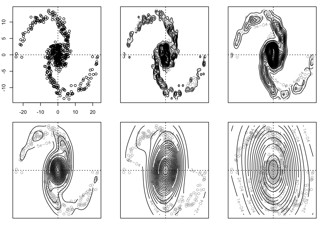
Figure 5.1 shows contours of the estimator \(\hat f_{n,h}\) computed on a simulated data set with \(d = 2\) at several choices of the bandwidth \(h\).

# bivariate kde function
biv_kde <- function(x,data,h){
  
  val <- mean(dnorm(data[,1] - x[1],0,h) * dnorm(data[,2]- x[2],0,h))
  return(val)
  
}

# generate bivariate data points that make a "galaxy"
n <- 500
a <- 1
b <- 1/2
theta <- runif(n,0,2*pi)
s <- sample(c(-1,1),n,replace = TRUE)
r <- s * a * exp(b * theta)

X <- matrix(0,n,2)
X[,1] <- r * cos(theta) + rnorm(n,0,1)
X[,2] <- r * sin(theta) + rnorm(n,0,1)

par(mfrow = c(2,3), mar = c(2.1,2.1,1.1,1.1))

# make a scatterplot of the data points
plot(X[,2] ~ X[,1],
     xlab = "",
     ylab = "")
abline(v = 0, lty = 3)
abline(h = 0, lty = 3)

# make contour plots of kdes at several choices of the bandwidth
hh <- c(1/2,1,2,4,8)
gridsize <- 120
x1 <- seq(min(X[,1]),max(X[,1]),length = gridsize)
x2 <- seq(min(X[,2]),max(X[,2]),length = gridsize)
zz <- matrix(0,gridsize,gridsize)
for( k in 1:length(hh)){
  
  plot(X[,2] ~ X[,1],
       xlab = "",
       ylab = "",
       xaxt = "n",
       yaxt = "n",
       col = "gray")
  abline( v = 0, lty = 3)
  abline( h = 0, lty = 3)
  
  zz <- matrix(0,gridsize,gridsize)
  for(i in 1:gridsize)
    for(j in 1:gridsize){
      
      zz[i,j] <- biv_kde(x = c(x1[i],x2[j]),data = X, h = hh[k])  
      
    }
  
  contour(x1, x2, zz, add = TRUE, nlevels = 20)
  
}

Figure 5.1: Contours of bivariate kernel density estimator at several bandwidths.