15 Implementing the bootstrap

Consider how to compute the bootstrap estimator \(\hat G_{Y_n}(x)\) of \(G_{Y_n}(x)\) for some \(x\). We have \[\begin{align} \hat G_{Y_n}(x) &= \mathbb{P}( Y_n^* \leq x|X_1,\dots,X_n)\\ &=\mathbb{P}(\sqrt{n}(\bar X_n^* - \bar X_n) \leq x|X_1,\dots,X_n)\\ &= \textstyle \mathbb{P}( \sum_{i=1}^n X_i^* \leq \sum_{i=1}^n X_i + \sqrt{n} x|X_1,\dots,X_n), \end{align}\] where, conditional on \(X_1,\dots,X_n\), the sum \(\sum_{i=1}^n X_i^*\) has a discrete distribution with as many as \(2n-1 \choose n\) atoms (think of putting \(n\) balls in as many urns).

It is possible to evaluate cumulative probabilities for \(\sum_{i=1}^nX_i^*|X_1,\dots,X_n\) exactly, but this can take too much time. We therefore almost always use Monte Carlo simulation to approximate the bootstrap estimator \(\hat G_{Y_n}\) of \(G_{Y_n}\) and its quantile function.

Definition 15.1 (Monte Carlo approximation to bootstrap estimator \(\hat G_{Y_n}\)) Choose a large \(B\). Then for \(b=1,\dots,B\) do:

Draw \(X_1^{*(b)},\dots,X_n^{*(b)}\) with replacement from \(X_1,\dots,X_n\).
Compute \(Y_n^{*(b)} =\sqrt{n}(\bar X_n^{*(b)} - \bar X_n)\), where \(\bar X^{*(b)} = n^{-1}\sum_{i=1}^n X_i^{*(b)}\).

Then set \(\hat G_{Y_n}(x) = B^{-1}\sum_{b=1}^B \mathbf{1}(Y_n^{*(b)} \leq x)\) for all \(x \in \mathbb{R}\).

We may call each sample \(X_1^{*(b)},\dots,X_n^{*(b)}\) in Definition 15.1 a bootstrap sample and each mean \(\bar X^{*(b)}\) a bootstrap mean.

Monte Carlo approximations to the quantiles \(\hat G^{-1}_{Y_n}(u)\) for \(u \in (0,1)\) may be obtained as follows: Sort the bootstrap realizations \(Y_n^{*(b)}\) from the Monte Carlo simulation such that \(Y_n^{*(1)} \leq \dots \leq Y_n^{*(b)}\) and then set \[ \hat G^{-1}_{Y_n}(u) = Y_n^{*(\lceil u B\rceil)} \] for all \(u \in (0,1)\). Note that the bootstrap confidence interval in Equation 14.3 can be constructed from the bootstrap means generated in the Monte Carlo simulation in Definition 15.1 as \[ \big[2\bar X_n - \bar X_n^{*(\lceil(1-\alpha/2)B \rceil)} , 2\bar X_n - \bar X_n^{*(\lceil(\alpha/2)B \rceil)} \big] \tag{15.1}\] after sorting them such that \(\bar X_n^{*(1)} \leq \dots \leq \bar X_n^{*(B)}\).

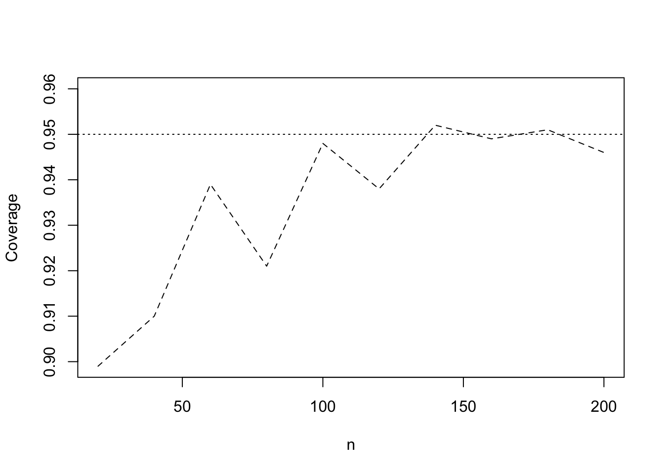
Figure 15.1 shows, over an increasing sample size \(n\), the realized coverage of the bootstrap interval in Equation 15.1 when the nominal coverage is set to \(1 - \alpha = 0.95\). Note that the coverage approaches the nominal level as the sample sizes increases.

Code

alpha <- 0.05
nn <- seq(20,200,by=20)
B <- 500
S <- 1000
shape <- 1.5
scale <- 4
mu <- shape * scale
zval <- qnorm(1 - alpha/2)

cvg <- numeric(length(nn))
for(j in 1:length(nn)){

  n <- nn[j]
  
  cov <- numeric(S)
  
  for(s in 1:S){

    X <- rgamma(n,shape = shape, scale = scale)
    Xbar <- mean(X)

    Xb <- matrix(X[sample(1:n,n*B,replace = TRUE)],n,B)
    Xbbar <- apply(Xb,2,mean)
    Xbbar_srt <- sort(Xbbar)

    lo <- 2*Xbar - Xbbar_srt[ceiling((1-alpha/2)*B)]
    up <- 2*Xbar - Xbbar_srt[ceiling(alpha/2*B)]
    cov[s] <- (lo < mu) & (up > mu)
  
  }

  cvg[j] <- mean(cov)
  
}

plot(NA,
     ylim = range(min(cvg),max(cvg,.96)),
     xlim = range(nn),
     xlab = "n",
     ylab = "Coverage")

lines(cvg ~ nn, lty = 2)
abline( h = 1 - alpha, lty = 3)

Figure 15.1: Coverage of confidence interval in Equation 15.1 with coverage probability set to \(1-\alpha = 0.95\) when \(X_1,\dots,X_n\) have the Gamma distribution with mean \(6\) and variance \(24\).

Why does the bootstrap work? Next we turn to theoretical guarantees.