7  The curse of dimensionality

$$

$$

In the previous section we derived an \(\operatorname{MSE}\) bound for a multivariate kernel density estimator (KDE) \(\hat f_{n,h}\) of an unknown density \(f:\mathbb{R}^d \to \mathbb{R}\) when the latter belongs to a class of Hölder functions with parameter \(\beta\) governing the smoothness. In particular, under the bandwidth \(h_{\operatorname{opt}}\) chosen to minimize the \(\operatorname{MSE}\), Proposition 6.3 gives the bound \[ \operatorname{MSE}\hat f_{n,h_{\operatorname{opt}}}(\mathbf{x}) \leq C^* n^{-2\beta/(2\beta + d)}, \tag{7.1}\] for all \(\mathbf{x}\in \mathbb{R}^d\). In this section we study the effect of \(d\) on the \(\operatorname{MSE}\) of \(\hat f_{n,h_{\operatorname{opt}}}\).

One way to understand the effect of the dimension \(d\) on the \(\operatorname{MSE}\) of our multivariate KDE is to suppose that a given \(\operatorname{MSE}\) bound has been achieved for \(d =1\) and then to find the sample sizes needed to achieve the same bound for dimensions \(d = 2,3,\dots\) That is, set up the inequality \[ C^*_d n_d^{-2\beta/(2\beta + d)} \leq C_1^*n_1^{-2\beta/(2\beta + 1)}, \] where \(C^*_1\) and \(C_d^*\) are constants and \(n_1\) and \(n_d\) are sample sizes in \(d = 1\) and \(d > 1\) settings, respectively, so that an \(\operatorname{MSE}\) bound of the form in Equation 7.1 appears on each side. Rearranging this, we obtain \[ n_d \geq \Big(\frac{C_d^*}{C_1^*}\Big)^{\frac{2\beta + d}{2\beta}} n_1^{\frac{2\beta + d}{2\beta + 1}}. \] The above equation shows that the sample size necessary to achieve, under higher dimensions \(d > 1\), the same \(\operatorname{MSE}\) bound as with sample size \(n_1\) when \(d = 1\) will be dramatically greater than \(n_1\).

For example, supposing \(\beta = 2\) (which would be the case, for example, if \(f\) has all partial derivatives of order \(2\), where these are bounded), ignoring the difference between the constants \(C_1^*\) and \(C_d^*\) (i.e. just setting \(C_1^* = C_d^*\)), and setting \(n_1 = 100\), we obtain in Table 7.1 the sample sizes \(n_d\), \(d = 2,\dots,8\) which would be necessary under these dimensions to achieve the same \(\operatorname{MSE}\) bound as in the \(d = 1\) setting with sample size \(n_1 = 100\). We see, for example, that if the dimension changes from \(d = 1\) to \(d = 3\), the sample size must be increased approximately six-fold to guarantee the same estimation accuracy; if the dimension increases from \(d = 1\) to \(d = 8\), an eight-fold increase, the sample size must be increased over six-hundred-fold!

Table 7.1: Sample size \(n_d\) needed (under \(\beta = 2\)) to achieve the same MSE bound for the multivariate KDE at dimensions \(d > 1\) as at \(d = 1\) with sample size \(n_1 = 100\).

\(d\)	1	2	3	4	5	6	7	8
\(n_d\)	100	251	631	1585	3981	10000	25119	63096

The requirement that to maintain the same estimation accuracy the sample size must increase exponentially in relation to the dimension has come to be referred to as the curse of dimensionality. How does the it arise? An observation that will help us understand how the curse of dimensionality arises is this: Points tend to be more “spread out” in higher dimensions. The next result, from Györfi et al. (2006), we should find compelling:

Proposition 7.1 (Points more thinly spread in higher dimensions) Let \(\mathbf{X},\mathbf{X}_1,\dots,\mathbf{X}_d \overset{\text{ind}}{\sim}\mathcal{U}([0,1]^d)\) for \(d \geq 1\). Then \[ \mathbb{E}\left[\min_{1\leq i\leq n} \|\mathbf{X}- \mathbf{X}_i\|_2\right] \geq \frac{d}{d+1}\left[\frac{\Gamma(d/2 + 1)^{1/d}}{\sqrt{\pi}}\right]\frac{1}{n^{1/d}}. \tag{7.2}\]

Proof of Proposition 7.1

We first write \[ \mathbb{E}\left[\min_{1\leq i\leq n} \|\mathbf{X}- \mathbf{X}_i\|_2\right] = \int_0^\infty[1 - \mathbb{P}(\min_{1\leq i\leq n} \|\mathbf{X}- \mathbf{X}_i\|_2 \leq t)]dt, \] and then seek a lower bound for the integrand on the right side. To this end, we write \[ \begin{align} \mathbb{P}(\min_{1\leq i\leq n} \|\mathbf{X}- \mathbf{X}_i\|_2 \leq t) & = \mathbb{P}(\|\mathbf{X}- \mathbf{X}_i\|_2 \leq t \text{ for at least one } i = 1,\dots,n )\\ & = \mathbb{P}( \cup_{i=1}^n \{\|\mathbf{X}- \mathbf{X}_i\|_2 \leq t \} )\\ & \leq n \mathbb{P}(\{\|\mathbf{X}- \mathbf{X}_1\|_2 \leq t ) \quad \text{ (by the union bound) }\\ & = n \int_{\{\mathbf{x}\in [0,1]^d\}}\int_{\{\mathbf{x}_1 \in [0,1]^d : \|\mathbf{x}_1 - \mathbf{x}\| \leq t\}} 1 d\mathbf{x}_1d\mathbf{x}\\ & \leq n \int_{\{\mathbf{x}\in [0,1]^d\}}\int_{\{\mathbf{x}_1 \in \mathbb{R}^d : \|\mathbf{x}_1 - \mathbf{x}\| \leq t\}} 1 d\mathbf{x}_1d\mathbf{x}\\ & = n\frac{\pi^{d/2}}{\Gamma(d/2 + 1)}t^d, \end{align} \] where we have used use fact that a ball in \(\mathbb{R}^d\) with radius \(t\) has volume given by \[ \int_{\{\mathbf{x}\in \mathbb{R}^d : \|\mathbf{x}\|_2 \leq t\}} 1 d\mathbf{x}= \frac{\pi^{d/2}}{\Gamma(d/2 + 1)}t^d. \] Now, considering \[ n\frac{\pi^{d/2}}{\Gamma(d/2 + 1)}t^d \leq 1 \iff t \leq \frac{1}{n^{1/d}}\frac{[\Gamma(d/2 + 1)]^{1/d}}{\pi^{d/2}}, \] the bound is only useful for \(t\) small enough, so we may write \[ 1 - \mathbb{P}(\min_{1\leq i\leq n} \|\mathbf{X}- \mathbf{X}_i\|_2 \leq t) \geq \left\{ \begin{array}{ll} 1 - n\frac{\pi^{d/2}}{\Gamma(d/2 + 1)}t^d,& \text{ if } t \leq \frac{1}{n^{1/d}}\frac{[\Gamma(d/2 + 1)]^{1/d}}{\pi^{d/2}}\\ 0, & \text{ otherwise.} \end{array}\right. \] The result is then given by writing \[ \mathbb{E}\left[\min_{1\leq i\leq n} \|\mathbf{X}- \mathbf{X}_i\|_2\right] \geq \int_0^{\frac{1}{n^{1/d}}\frac{[\Gamma(d/2 + 1)]^{1/d}}{\pi^{d/2}}}\Big(1 - n\frac{\pi^{d/2}}{\Gamma(d/2 + 1)}t^d\Big)dt. \] and evaluating the integral on the right side.

Proposition 7.1 posits a situation in which some random points \(\mathbf{X}_1,\dots,\mathbf{X}_n\) are uniformly drawn on the hypercube \([0,1]^d\), after which an additional point \(\mathbf{X}\) is drawn on the same hypercube and the question is asked, “what is the distance from \(\mathbf{X}\) to the nearest point among \(\mathbf{X}_1,\dots,\mathbf{X}_n\)?”. The result says that the expected value of this distance decreases with \(n\), but the rate of this decrease is affected by the dimension \(d\) such that for larger \(d\), the decrease with respect to \(n\) is (much) slower. An interpretation of this is that it takes many more points \(\mathbf{X}_1,\dots,\mathbf{X}_n\) to “fill up” a high-dimensional space (large \(d\)) than a low dimensional space (small \(d\)).

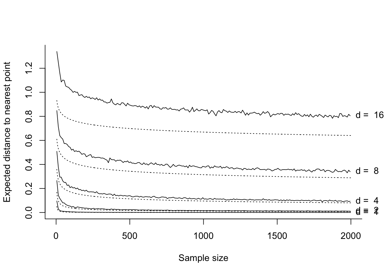
Figure 7.1 plots the lower bound given on the right side of Equation 7.2 (dotted lines) over a sequence of sample sizes \(n\) for several dimensions \(d\) as well as Monte Carlo approximations to the mean distances on the left side of Equation 7.2 (solid lines). The bound appears not to be very tight for high dimensions, yet it reflects nonetheless convincingly the curse of dimensionality.

dd <- 2^(0:4)
nn <- seq(5,2000,by = 10)
S <- 100
md <- array(0,dim = c(length(nn),length(dd),S))
for(j in 1:length(dd))
  for(i in 1:length(nn))
    for(s in 1:S){
    
      U <- runif(dd[j]*(nn[i]+1),0,1)
      X <- matrix(U,nn[i]+1,dd[j])
      D <- matrix(1,nn[i],1) %*% X[1,] - X[-1,]
      md[i,j,s] <- min(sqrt(apply(D^2,1,sum)))
    
    }
  
Emd <- apply(md,c(1,2),mean)


plot(NA,
     ylim = range(Emd),
     xlim = range(nn),
     xlab = "Sample size",
     ylab = "Expected distance to nearest point",
     bty = "l")

nn2 <- 5:2000
Emd_lo <- matrix(0,length(nn2),length(dd))

for(j in 1:length(dd)){
  
  Emd_lo[,j] <- dd[j]/(dd[j]+1)*gamma(dd[j]/2 + 1)^(1/dd[j])/sqrt(pi)*nn2^(-1/dd[j])
  
}

for(j in 1:length(dd)){
  
  lines(Emd[,j]~nn)
  lines(Emd_lo[,j]~nn2, lty=3)
  text(x = max(nn), y = Emd[length(nn),j], paste( "d = ", dd[j]), pos = 4, xpd = NA)
  
}

Figure 7.1: Simulation illustrating Proposition 7.1. Solid lines: Simulated average distance to nearest point. Dotted lines: Lower bound on the expected distance.

The relation this has to density estimation is that, in order to estimate a density \(f\) with a certain accuracy at a point \(\mathbf{x}\in \mathbb{R}^d\), one must have a sufficient number of observations in a small neighborhood of \(\mathbf{x}\). As the dimension \(d\) increases, the number of observations in any neighborhood of fixed volume will tend to decrease, leading to a dramatic inflation of the variance of our multivariate KDE (which can only be countered by exponentially increasing the sample size as the dimension grows).

Györfi, László, Michael Kohler, Adam Krzyzak, and Harro Walk. 2006. A Distribution-Free Theory of Nonparametric Regression. Springer Science & Business Media.