Here we present some examples of Edgeworth expansions in order to demonstrate their ability to approximate the sampling distribution of the standardized pivot \(Z_n = \sqrt{n}(\bar X_n - \mu)/\sigma\) as well as that of the studentized pivot \(T_n = \sqrt{n}(\bar X_n - \mu) /S_n\).
32.1 For the standardized pivot
We first consider the case of the standardized pivot \(Z_n = \sqrt{n}(\bar X_n - \mu)/\sigma\). We begin by defining, following the proof of Theorem 31.1, the first-order Edgeworth expansions of the cdf \(F_{Z_n}\) and the pdf \(f_{Z_n}\) of \(Z_n\) as \[\begin{align}
\tilde F^{(1)}_{Z_n}(z) &\equiv \Phi(z) - \frac{1}{6\sqrt{n}}\frac{\mu_3}{\sigma^3}(z^2 - 1)\phi(z)\\
\tilde f^{(1)}_{Z_n}(z) &\equiv \phi(z) + \frac{1}{6\sqrt{n}}\frac{\mu_3}{\sigma^3}(z^3 - 3z)\phi(z)
\end{align}\] and their second-order counterparts as \[\begin{align}
\tilde F_{Z_n}^{(2)}(z) &\equiv \tilde F_{Z_n}^{(1)}(z) - \frac{1}{n}\Big[\frac{1}{24}\Big(\frac{\mu_4}{\sigma^4} - 3\Big)(z^3 - 3z) + \frac{1}{72}\frac{\mu_3^2}{\sigma^6}(z^5 - 10z^3 + 15z)\Big]\phi(z)\\
\tilde f_{Z_n}^{(2)}(z) &\equiv \tilde f_{Z_n}^{(1)}(z) + \frac{1}{n}\Big[\frac{1}{24}\Big(\frac{\mu_4}{\sigma^4} - 3\Big)(z^4 - 6z^2 + 3) + \frac{1}{72}\frac{\mu_3^2}{\sigma^6}(z^6 - 15z^4 + 45z^2 - 15)\Big]\phi(z).
\end{align}\] We may also regard \[\begin{align}
\tilde F^{(0)}_{Z_n}(z) &\equiv \Phi(z)\\
\tilde f^{(0)}_{Z_n}(z) &\equiv \phi(z)
\end{align}\] as Edgeworth expansions of order zero.
We are interested in checking how close the approximations \(\tilde F^{(j)}_{Z_n}\) and \(\tilde f^{(j)}_{Z_n}\) are to the exact cdf \(F_{Z_n}\) and exact pdf \(f_{Z_n}\), respectively, of \(Z_n\) for orders \(j=0,1,2\) in finite-\(n\) settings.
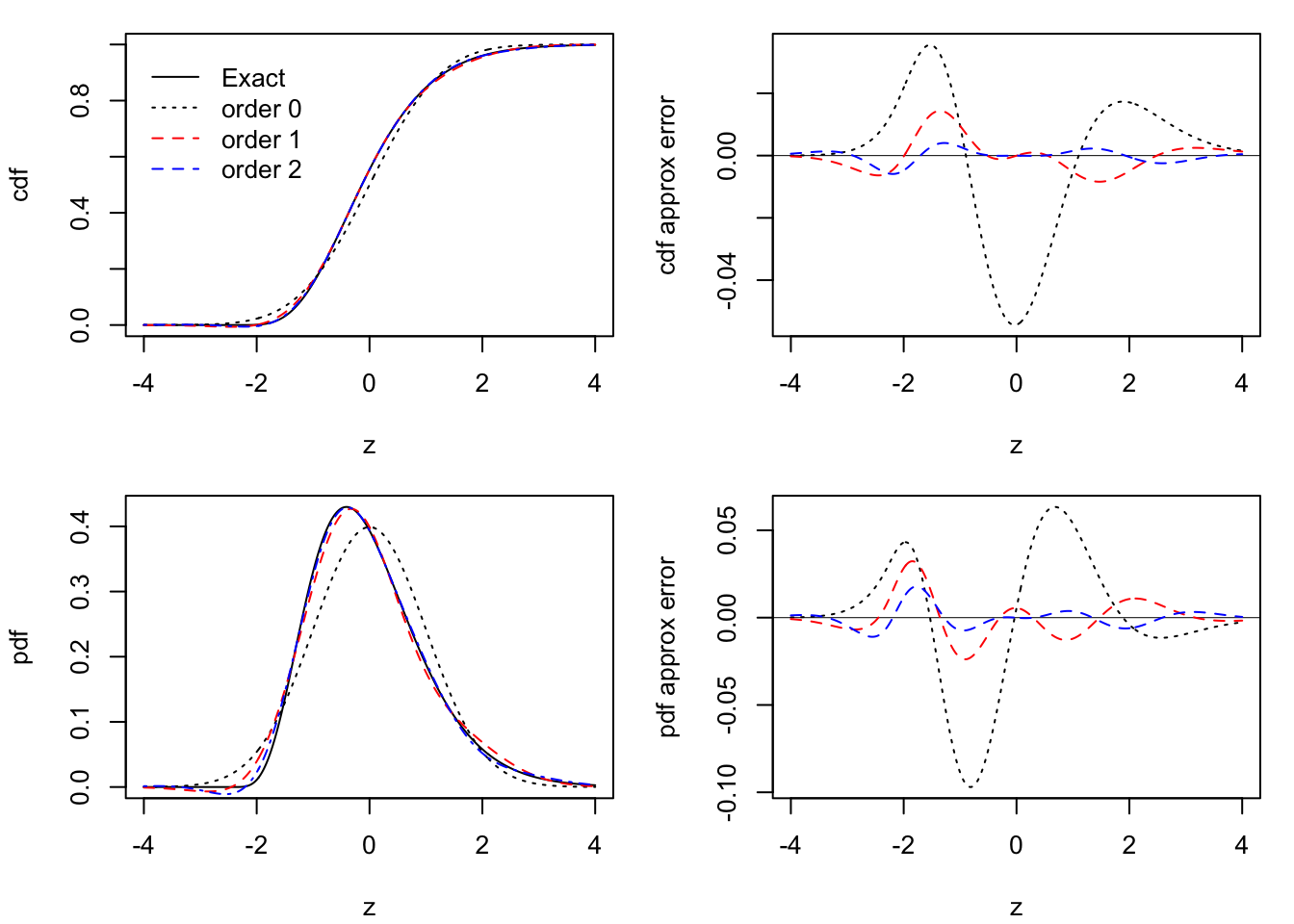
Example 32.1 Let \(X_1,\dots,X_n\) be independent random variables having the exponential distribution with mean \(\lambda\). Since \(\mathbb{E}X_1 = \lambda\) and \(\mathbb{V}X_1 = \lambda^2\), the studentized pivot \(Z_n\) is given by \(Z_n = \sqrt{n}(\bar{X}_n - \lambda) / \lambda\). This random variable has, for each \(n\geq 1\), the \(\mathcal{G}(n,n^{-1/2})\) distribution centered to have mean zero, where \(\mathcal{G}(a,b)\) denotes the Gamma distribution with mean \(ab\) and variance \(ab^2\). The density of \(Z_n\) is therefore given by \[
f_{Z_n}(z) = \frac{1}{\Gamma(n)(1/\sqrt{n})^n}(z+\sqrt{n})^{n-1}\exp\left(-\frac{z +\sqrt{n}}{1/\sqrt{n}}\right)\mathbf{1}(z > -\sqrt{n}).
\] Based on the moments of the exponential distribution, we find \(\mu_3/\sigma^3 = 2\) and \(\mu_4/\sigma^4 = 9\), with which the first- and second-order Edgeworth expansions can be defined.
Figure 32.1 overlays the cdfs \(F_{Z_n}\) and \(\tilde F_{Z_n}^{(j)}\) for \(j=0,1,2\) as well as the pdfs \(f_{Z_n}\) and \(\tilde f_{Z_n}^{(j)}\) for \(j=0,1,2\) and plots the approximation errors of the expansions. We see that the first-order Edgeworth expansion provides a much better approximation to the true distribution of \(Z_n\) than the asymptotic \(\mathcal{N}(0,1)\) distribution (which is the order-0 Edgeworth expansion). The second-order Edgeworth expansion does not appear to improve much on the quality of the first-order expansion.
Code
# define needed HermitepolynomialsH2 <-function(z){z^2-1}H3 <-function(z){z^3-3*z}H4 <-function(z){z^4-6*z^2+3}H5 <-function(z){z^5-10*z^3+15*z}H6 <-function(z){z^6-15*z^4+45*z^2-15}# input values of gamma and taugam <-2tau <-9# choose a sample sizen <-6# get exact pdf and cdfz <-seq(-4, 4, length =500)fz <-dgamma(z +sqrt(n),shape = n, scale =1/sqrt(n))Fz <-pgamma(z +sqrt(n),shape = n, scale =1/sqrt(n))# get Edgeworth expansionsF0z <-pnorm(z)f0z <-dnorm(z)F1z <-pnorm(z) -dnorm(z)*gam/6*H2(z)/sqrt(n)f1z <-dnorm(z) +dnorm(z)*gam/6*H3(z)/sqrt(n)F2z <- F1z -dnorm(z)*((tau -3)/24*H3(z) + gam^2/72*H5(z)) / nf2z <- f1z +dnorm(z)*((tau -3)/24*H4(z) + gam^2/72*H6(z)) / n# make plotspar(mfrow =c(2,2), mar =c(4.1,4.1,1.1,1.1))# cdf approximationplot(Fz ~ z, type ="l",ylab ="cdf")lines(F0z ~ z, lty =3)lines(F1z ~ z, lty =2, col ="red")lines(F2z ~ z, lty =4, col ="blue")xpos <-grconvertX(x = .2,from="nfc", to ="user")ypos <-grconvertY(y = .9,from="nfc", to ="user")legend(x = xpos,y = ypos,legend =c("Exact","order 0","order 1","order 2"),lty =c(1,3,2,2),col =c("black","black","red","blue"),bty="n")# cdf approximation errorplot(F0z - Fz ~ z, type ="l",lty =3,ylab ="cdf approx error")abline(h =0,lwd= .5)lines(F1z - Fz ~ z, lty =2, col ="red")lines(F2z - Fz ~ z, lty =2, col ="blue")# pdf approximationplot(fz ~ z, type ="l",ylab ="pdf")lines(f0z ~ z, lty =3)lines(f1z ~ z, lty =2, col ="red")lines(f2z ~ z, lty =4, col ="blue")# pdf approximation errorplot(f0z - fz ~ z, type ="l",lty =3,ylab ="pdf approx error")abline(h =0,lwd= .5)lines(f1z - fz ~ z, lty =2, col ="red")lines(f2z - fz ~ z, lty =2, col ="blue")
Figure 32.1: Quality of Edgeworth expansions of order 0, 1, and 2 for the distribution of \(Z_n\) when \(X_1,\dots,X_n\) have the exponential distribution. Results shown for the sample size \(n = 6\).
32.2 For the studentized pivot
Now we consider the studentized pivot \(T_n = \sqrt{n}(\bar X_n - \mu) /S_n\). As in the previous section, we will begin by defining first- and second-order Edgeworth expansions, but this time according to Theorem 31.2. Let the first-order Edgeworth expansions of the cdf \(F_{T_n}\) and the pdf \(f_{T_n}\) of \(T_n\) be defined as \[\begin{align}
\hat F^{(1)}_{T_n}(t) &\equiv \Phi(t) + \frac{1}{6\sqrt{n}}\frac{\mu_3}{\sigma^3}(2t^2 + 1)\phi(t)\\
\hat f^{(1)}_{T_n}(t) &\equiv \phi(t) - \frac{1}{6\sqrt{n}}\frac{\mu_3}{\sigma^3}(2t^3 - 3t)\phi(t)
\end{align}\] and their second-order counterparts as \[\begin{align}
\hat F_{T_n}^{(2)}(t) &\equiv \hat F_{T_n}^{(1)}(t) + \frac{1}{n}\Big[\frac{1}{12}\Big(\frac{\mu_4}{\sigma^4} - 3\Big)(t^3 - 3t) - \frac{1}{18}\frac{\mu_3^2}{\sigma^6}(t^5 + 2t^3 - 3t) - \frac{1}{4}(t^3 + 3t)\Big]\phi(t)\\
\hat f_{T_n}^{(2)}(t) &\equiv \hat f_{T_n}^{(1)}(t) - \frac{1}{n}\Big[\frac{1}{12}\Big(\frac{\mu_4}{\sigma^4} - 3\Big)(t^4 - 6t^2 + 3) - \frac{1}{18}\frac{\mu_3^2}{\sigma^6}(t^6 -3t^4 - 9t^2 + 3) - \frac{1}{4}(t^4 - 3)\Big]\phi(t),
\end{align}\] where the pdf approximations may be obtained by taking differentiating the corresponding cdf approximation. As before we may also regard \[\begin{align}
\hat F^{(0)}_{T_n}(t) &\equiv \Phi(t)\\
\hat f^{(0)}_{T_n}(t) &\equiv \phi(t)
\end{align}\] as Edgeworth expansions of order zero.
We are interested in checking how close the approximations \(\hat F^{(j)}_{Z_n}\) and \(\hat f^{(j)}_{Z_n}\) are to the exact cdf \(F_{Z_n}\) and exact pdf \(f_{Z_n}\), respectively, of \(Z_n\) for orders \(j=0,1,2\) in finite-\(n\) settings.
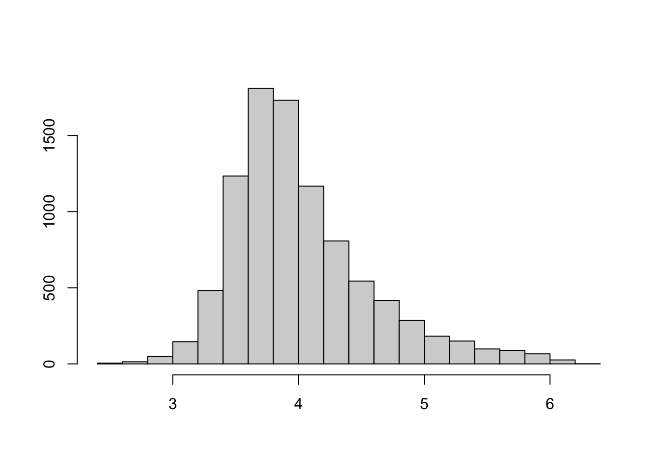
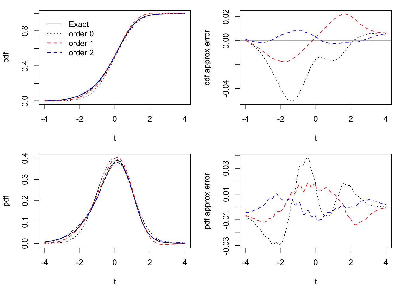
Example 32.2 To assess the quality of the Edgeworth approximations for the studentized pivot, we run a simulation in which we treat the women’s finishing times for the 2009 Boston Marathon as a population and repeatedly draw random samples of size \(n\).
Code
# not sure where I want to store this file in the long run...load(url("https://people.stat.sc.edu/gregorkb/data/bos09whrs.Rdata"))hist(bos09whrs, main ="", ylab ="", xlab ="")N <-length(bos09whrs)mu <-mean(bos09whrs)sigma <-sqrt(mean((bos09whrs - mu)^2))gamma <-mean( (bos09whrs - mu)^3) /sigma^3tau <-mean( (bos09whrs - mu)^4) /sigma^4# choose a sample size and number of simulationsn <-15S <-100000
Figure 32.2: Histogram of finishing times (in hours) of 9303 women in the 2009 Boston Marathon.
The empirical distribution of the 9303 finishing times has \(\mu_3/\sigma^3 = 1.09\) and \(\mu_4/\sigma^4 = 4.41\). Under \(n = 15\), we obtain an approximation to the true pdf and cdf of \(T_n = \sqrt{n}(\bar{X}_n - \mu)/S_n\) with a kernel density estimator based on \(10^{5}\) simulated samples. Then we compare the kernel density estimate of the pdf and cdf to the Edgeworth expansions of orders \(j=0,1,2\).
Code
X <-matrix(bos09whrs[sample(N,S*n,replace=TRUE)],S,n)Tn <-sqrt(n)*(apply(X,1,mean) - mu)/apply(X,1,sd)kde <-density(Tn,from =-4,to =4)ft <- kde$yFt <-c(0,cumsum(kde$y[-1]*diff(kde$x)))t <- kde$xf0t <-dnorm(t)F0t <-pnorm(t)F1t <-pnorm(t) +dnorm(t) * gamma / (6*sqrt(n)) * (2*t^2+1)f1t <-dnorm(t) * ( 1- gamma / (6*sqrt(n)) * (2*t^3-3*t))F2t <- F1t +dnorm(t)*((tau -3)/12*(t^3-3*t) - gamma^2/18*(t^5+2*t^3-3*t) -1/4*(t^3+3*t))/nf2t <- f1t -dnorm(t)*((tau -3)/12*(t^4-6*t^2+3) - gamma^2/18*(t^6-3*t^4-9*t^2+3) -1/4*(t^4-3))/n# make plotspar(mfrow =c(2,2), mar =c(4.1,4.1,1.1,1.1))plot(Ft ~ t, type ="l",ylab ="cdf")lines(F0t ~ t, lty =3)lines(F1t ~ t, lty =2, col ="red")lines(F2t ~ t, lty =4, col ="blue")xpos <-grconvertX(x = .2,from="nfc", to ="user")ypos <-grconvertY(y = .9,from="nfc", to ="user")legend(x = xpos,y = ypos,legend =c("Exact","order 0","order 1","order 2"),lty =c(1,3,2,2),col =c("black","black","red","blue"),bty="n")# cdf approximation errorylims <-range(F0t - Ft,F1t - Ft,F2t - Ft)plot(F0t - Ft ~ t, ylim = ylims,type ="l",lty =3,ylab ="cdf approx error")abline(h =0,lwd= .5)lines(F1t - Ft ~ t, lty =2, col ="red")lines(F2t - Ft ~ t, lty =2, col ="blue")# pdf approximationylims <-range(ft,f0t,f1t,f2t)plot(ft ~ t, ylim = ylims,type ="l",ylab ="pdf")lines(f0t ~ t, lty =3)lines(f1t ~ t, lty =2, col ="red")lines(f2t ~ t, lty =4, col ="blue")# pdf approximation errorplot(f0t - ft ~ t, type ="l",lty =3,ylab ="pdf approx error")abline(h =0,lwd= .5)lines(f1t - ft ~ t, lty =2, col ="red")lines(f2t - ft ~ t, lty =2, col ="blue")
We notice, again, that the first- and second-order Edgeworth expansions are of similar quality and that they provide better approximations to the sampling distribution of \(T_n\) than the asymptotic \(\mathcal{N}(0,1)\) distribution, i.e. the order-0 Edgeworth expansion.
Next we take a brief foray into multivariate Edgeworth expansions.