8Nonparametric regression with the Nadaraya-Watson estimator
$$
$$
Suppose we observe covariate and response data \((x_1,Y_1),\dots,(x_n,Y_n)\in [0,1] \times \mathbb{R}\), where \[
Y_i = m(x_i) + \varepsilon_i,
\]\(i = 1,\dots,n\), where \(m:[0,1] \to \mathbb{R}\) is an unknown function and \(\varepsilon_1,\dots,\varepsilon_n\) are independent random variables with mean \(0\) and variance \(\sigma^2\).
Here, for each \(i=1,\dots,n\), \(Y_i\) represents a response value and \(x_i\) a covariate value. We note that the interval \([0,1]\) is arbitrary and chosen for convenience (one can always rescale the observed covariate values to lie in this interval). We will for the most part treat \(x_1,\dots,x_n\) as deterministic, that is, not as random variables, since in most regression contexts one usually conditions on the observed covariate values. We will sometimes refer to \(x_1,\dots,x_n\) as the set of design points.
Our aim is to estimate the unknown function \(m\) without making assumptions about its shape. Our development will follow closely Section 1.5 of Tsybakov (2008).
Parametric regression methods assume a functional form for \(m\) such that \(m\) is determined by a finite number of parameters. For example, simple linear regression assumes \(m\) takes the form \(m(x) = \beta_0 + \beta_1 x\) for some intercept and slope parameters \(\beta_0,\beta_1\in \mathbb{R}\), so that one may estimate \(m\) simply by estimating the values of the two parameters \(\beta_0\) and \(\beta_1\). In contrast, nonparametric regression methods, assume only that \(m\) belongs to some class of functions, for example \(m \in \text{Lipschitz}(L,[0,1])\); see Definition 2.1.
There are myriad ways to estimate an unknown function “nonparametrically”, that is, without assuming a parametric form for \(m\). In this section we will focus on the Nadaraya-Watson estimator, which can be concieved as a generalization of the most rudimentary estimator in nonparametric regression—the local average estimator, which is given, for some \(h>0\), by \[
\bar m_{n,h}(x) = \frac{\sum_{i=1}^n Y_i \cdot \mathbb{I}(x - h \leq x_i \leq x + h)}{\sum_{j=1}^n \mathbb{I}(x - h \leq x_j \leq x + h)}
\] for all \(x\), where \(\mathbb{I}\) is an indicator function. This estimator computes, for each \(x\), the mean of the response values \(Y_i\) for which the covariate value \(x_i\) lies within a distance \(h>0\) of \(x\).
The Nadaraya-Watson estimator generalizes the local average estimator by allowing the specification of a kernel function \(K\) designed to place greater weight on observations for which \(x_i\) is closer to \(x\), and to allow the weight to decay smoothly to zero as \(x_i\) is further from \(x\).
Definition 8.1 (The Nadaraya-Watson estimator) For some kernel function \(K:\mathbb{R}\to \mathbb{R}\) and bandwidth \(h>0\), the Nadaraya-Watson estimator is given by \[
\hat m_{n,h}^{\operatorname{NW}}(x) = \frac{\sum_{i=1}^n Y_iK((x_i - x)/h)}{\sum_{j=1}^nK((x_j - x)/h)}
\] for all \(x\).
Note that under \(K(u) = (1/2)\mathbb{I}(u \in[-1,1])\), the Nadaraya-Watson estimator becomes the local-average estimator. Typically \(K\) is chosen as a density, just as in kernel density estimation.
Note that when \(K\) has bounded support, \(\hat m_{n,h}^{\operatorname{NW}}(x)\) may be undefined for some \(x\); for example, the local-average estimator will be undefined at \(x\) if there are no covariate values \(x_i\) within the distance \(h\) of \(x\). Choosing \(K\) to be, for example, the Gaussian kernel, which has support on all of \(\mathbb{R}\), ensures that the Nadaraya-Watson estimator is defined for all \(x\). One can also simply increase the bandwidth. In establishing \(\operatorname{MSE}\) bounds later on, we will find it convenient to assume the kernel has support only on \([-1,1]\), as in the case of the local-average kernel.
Otherwise than as a generalization of the local-average estimator, we can understand the Nadaraya-Watson estimator as computing the conditional mean of \(Y_i\) when \(x_i = x\) according to a kernel density estimate of the conditional distribution. That is, letting \[
\begin{align}
\hat f_{n,h}(x) &= \frac{1}{nh}\sum_{i=1}^nK\Big(\frac{x_i- x}{h}\Big) \\
\hat f_{n,h}(x,y) & = \frac{1}{nh^2}\sum_{i=1}^nK\Big(\frac{Y_i - y}{h}\Big)K\Big(\frac{x_i- x}{h}\Big)
\end{align}
\tag{8.1}\] for all \(x,y\), and then setting \(\hat f_{n,h}(y|x) = \hat f_{n,h}(x) / \hat f_{n,h}(x,y)\), we have \[
\hat m_{n,h}^{\operatorname{NW}}(x) = \int_\mathbb{R}y \hat f_{n,h}(y|x)dy,
\tag{8.2}\] provided the kernel \(K\) satisfies \(\int_\mathbb{R}K(u)du = 1\) and \(\int_\mathbb{R}u K(u)du = 0\).
We may write \[
\begin{align}
\int_\mathbb{R}y \hat f_{n,h}(y|x)dy &= \frac{1}{\hat f_{n,h}(x)}\int_\mathbb{R}y \hat f_{n,h}(x,y)dy\\
&= \frac{1}{\hat f_{n,h}(x)}\sum_{i=1}^n K((x_i- x)/h)\frac{1}{h}\int_\mathbb{R}y K((Y_i - y)/h)dy \\
&= \frac{\sum_{i=1}^n Y_iK((x_i - x)/h)}{\sum_{j=1}^nK((x_j - x)/h)},
\end{align}
\] since for each \(i=1,\dots,n\) we have \[
\frac{1}{h}\int_\mathbb{R}y K((Y_i - y)/h)dy = \int_\mathbb{R}(Y_i - uh)K(u)du = Y_i,
\] by the assumptions on the kernel \(K\).
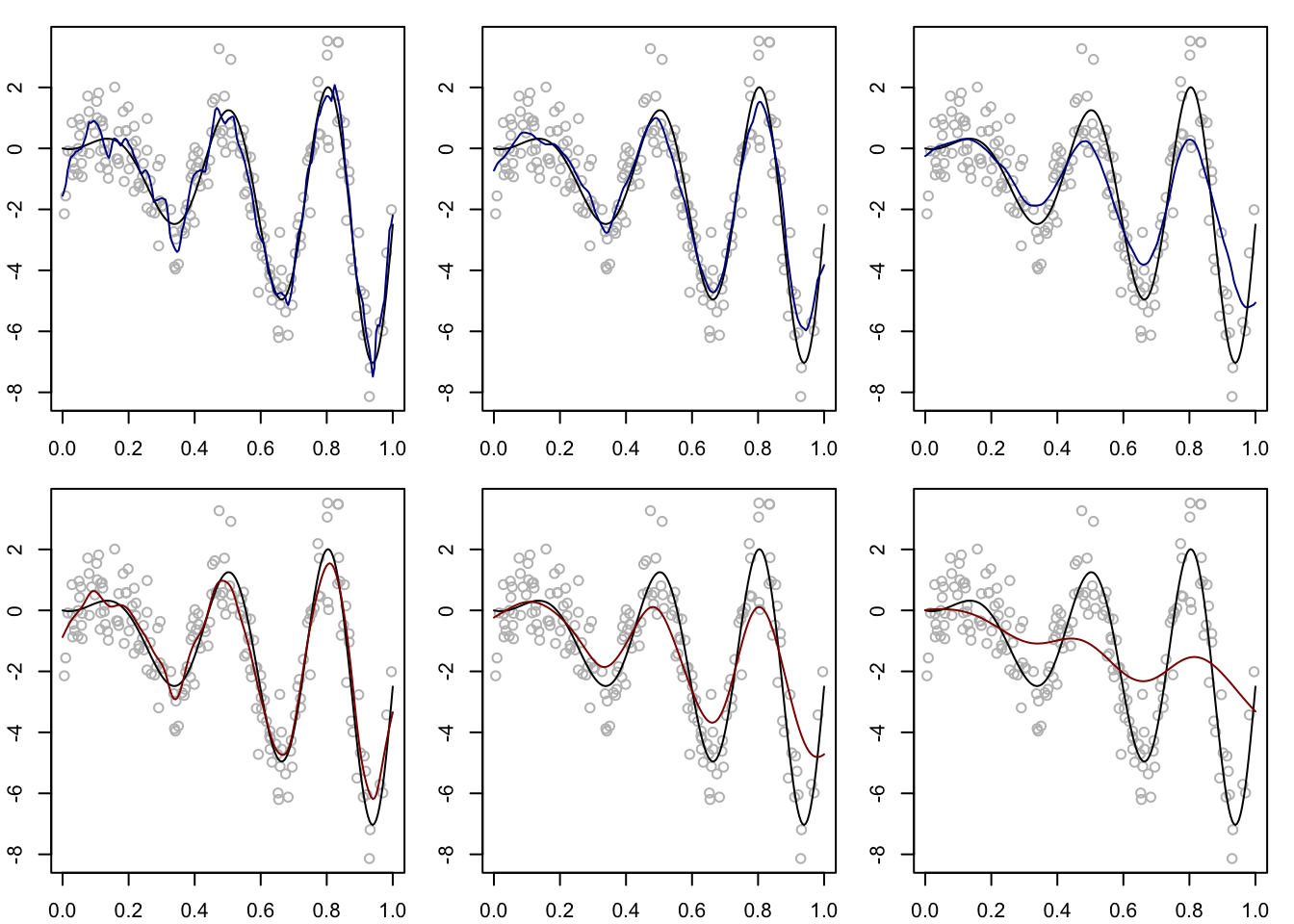
Figure 8.1 shows the Nadaraya-Watson estimator computed on a synthetic data set under two different choices of the kernel \(K\) and under three choices of the bandwidth \(h\).
Code
# Epanechnikov kernelepker <-function(x){3/4*(1- x^2) *((x <=1) & (x >=-1)) }# NW estimatormNW <-function(x,data,K,h){ Wx <-K((data$X - x)/h) /sum(K((data$X - x)/h)) mNWx <-sum(Wx*data$Y)return(mNWx)}# true function mm <-function(x) 5*x*sin(2*pi*(1+ x)^2) - (5/2)*x# generate datan <-200X <-runif(n)e <-rnorm(n)Y <-m(X) + edata <-list(X = X,Y = Y)# plot NW estimator at two choices of kernel and three choices of bandwidthpar(mfrow =c(2,3), mar=c(2.1,2.1,1.1,1.1))x <-seq(0,1,length=200)hh <-c(0.02,0.05,0.10)KK <-list(epker, dnorm)cols <-c(rgb(0,0,.545,1),rgb(0.545,0,0,1))for(k in1:2)for(j in1:3){ mNWx <-sapply(x,FUN=mNW,data=data,h=hh[j],K=KK[[k]])plot(Y~X, col ="gray")lines(m(x)~x)lines(mNWx~x,col=cols[k])}
Figure 8.1: Nadaraya-Watson estimator under two choices of the kernel function \(K\) (top row Epanechnikov, bottom row Gaussian), and three choices of the bandwith \(h\) (increasing from left to right) on a synthetic data set.
Tsybakov, Alexandre B. 2008. Introduction to Nonparametric Estimation. Springer Science & Business Media.