In order to study the capability of the bootstrap to estimate sampling distributions of statistics apart from the sample mean, we discuss what are called statistical functionals. For an authoritative and thorough monograph on statistical functionals and von Mises expansions (which we discuss in this section), the reader is referred to Fernholz (2012), upon which these notes heavily rely.
Definition 36.1 (Statistical functional) A statistical functional is a function \(T:\mathcal{D}\to \mathbb{R}\), where \(\mathcal{D}\) is the space of probability distributions.
Assume \(X_1,\dots,X_n\) are independent, identically distributed random variables having distribution \(F \in \mathcal{D}\). Then we will be interested in estimating and making inferences on a parameter \(\theta\) defined according to statistical functional \(T\) applied to \(F\). That is, we consider estimating the parameter \[
\theta = T(F).
\] As an estimator of \(\theta\), we consider the estimator \(\hat \theta_n\) obtained by plugging the empirical cdf \(\hat F_n\) into the functional \(T\). That is \[
\hat \theta_n = T(\hat F_n),
\] where \(\hat F_n\) is the distribution placing mass \(1/n\) at each \(X_1,\dots,X_n\). We call this the plug-in estimator.
With some abuse of notation, we will use \(F\) or \(\hat F_n\) to represent either a distribution in \(\mathcal{D}\) or its cdf. For example, we may write the empirical distribution \(\hat F_n\) of \(X_1,\dots,X_n\) as \[
\hat F_n = n^{-1}\sum_{i=1}^n \delta_{X_i},
\] where \(\delta_x\) is the Dirac measure—the discrete distribution placing unit mass on the point \(x\)—and we may also write the cdf of the distribution \(\hat F_n\) as \[
\hat F_n(x) = n^{-1}\sum_{i=1}^n \mathbf{1}(x_i \leq x)
\] for \(x \in \mathbb{R}\).
The intuition behind the plug-in estimator is that, since \(\hat F_n\) is a good estimator of \(F\), we hope that \(T(\hat F_n)\) will be a good estimator \(T(F)\). We find, as may be expected, that we will need certain conditions on the functional \(T\) in order for the plug-in estimator to have nice properties such as consistency or asymptotic Normality. Before discussing any of these conditions, we introduce some examples of statistical functions in Table 36.1 (it is a good exercise to derive the expressions for the plug-in estimators).
Table 36.1: Examples of statistical functionals and corresponding plug-in estimators
In order to make inferences on a statistical functional \(\theta = T(F)\) based on the plug-in estimator \(\hat \theta_n = T(\hat F_n)\), we will rely on some results that give conditions under which \[
\sqrt{n}(T(\hat F_n) - T(F)) \stackrel{d}{\rightarrow}\mathcal{N}(0,\sigma_T^2),
\tag{36.1}\] as \(n \to \infty\) for some variance \(\sigma_T^2\). To obtain such a result, we will consider something akin to a Taylor expansion of \(T\) around \(F\) evaluated at \(\hat F_n\). In order to obtain such an expansion of \(T\), we need the notion of a derivative of a function which maps probability distributions to real numbers. This notion is formalized in the von Mises derivative of a statistical functional.
Definition 36.2 (von Mises derivative of a statistical functional) The von Mises derivative of \(T\) at \(F\) in the direction of \(G\) is defined as \[
T^{(1)}_F(G-F) = \frac{d}{d\epsilon} T(F + \epsilon(G - F))\Big|_{\epsilon = 0},
\] provided there exists a function \(\varphi_F\), not depending on \(G\), such that \[
\frac{d}{d\epsilon} T(F + \epsilon(G - F))\Big|_{\epsilon = 0} = \int \varphi_F(x) d(G - F)(x)
\tag{36.2}\] with \(\int \varphi_F(x) dF(x) = 0\).
Definition 36.3 (Influence curve) The function \(\varphi_F\) in Equation 36.2, provided it exists, is called the influence curve of the functional \(T\) at \(F\) and is given by \[
\varphi_F(x) = \frac{d}{d\epsilon}T(F + \epsilon(\delta_x-F))\Big|_{\epsilon=0}.
\tag{36.3}\]
We show that the expression in Equation 36.3 satisfies the condition in Equation 36.2. We have \[\begin{align}
\int \frac{d}{d\epsilon}&T(F + \epsilon(\delta_x-F))\Big|_{\epsilon=0} d(G - F)(x) \\
&= \frac{d}{d\epsilon}\Big[ \int T(F + \epsilon(\delta_x-F)) dG(x) - \int T(F + \epsilon(\delta_x-F)) dF(x) \Big]\Big|_{\epsilon = 0}\\
&= \frac{d}{d\epsilon}\Big[ T(F + \epsilon(G-F)) - T(F + \epsilon(F-F)) \Big]\Big|_{\epsilon = 0}\\
&=\frac{d}{d\epsilon}T(F + \epsilon(G-F))\Big|_{\epsilon = 0}.
\end{align}\]
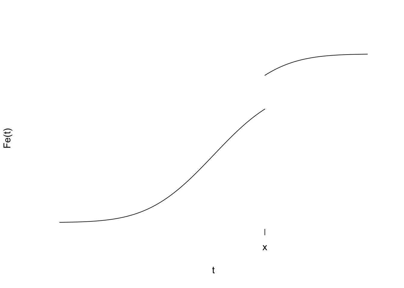
The influence curve \(\varphi_F\) measures the change in \(T(F)\) when \(F\) is perturbed by the addition of a point mass at \(x\). Influence curves play an important role in the study of robust estimation when one considers the effect of outliers, for example.
The Taylor-like expansion we have alluded to which will help us to obtain an asymptotic Normality result like that in Equation 36.1 will make use of the von Mises derivative, having the form \[
T(\hat F_n) = T(F) + T^{(1)}_F(\hat F_n - F) + R_F(\hat F_n - F),
\tag{36.4}\] where \(T^{(1)}_F(\hat F_n - F)\) is the von Mises derivative of \(T\) at \(F\) in the direction of \(\hat F_n\) and \(R_F(\hat F_n - F)\) is a remainder term. Key to the asymptotic Normality result is the fact that \(T^{(1)}_F(\hat F_n - F)\) can be written as the mean of \(n\) independently, identically distributed random variables. In particular, we have \[
T^{(1)}_F(\hat F_n - F) = \frac{1}{n}\sum_{i=1}^n \varphi_F(X_i)
\tag{36.5}\] so that the von Mises derivative of \(T\) at \(F\) in the direction of \(\hat F_n\) can be written as the mean of the influence function over the observed data points \(X_1,\dots,X_n\).
From here, using our von Mises expansion in Equation 36.4, we may write \[
\sqrt{n} (T(\hat F_n) - T(F)) = \frac{1}{\sqrt{n}}\sum_{i=1}^n \varphi_F(X_i) + \sqrt{n} R_F(\hat F_n - F),
\] where we intend that first term on the right hand side should converge to a Normal limit and that the second should vanish for large \(n\). Setting \[
\sigma_T^2 = \int\varphi_F^2(x)dF(x)
\] provided this is finite and that the remainder term indeed vanishes, leads to the desired asymptotic Normality expressed in Equation 36.1. Note that \(\int\varphi_F^2(x)dF(x) = \mathbb{V}\varphi_F(X_1)\) since \(\int\varphi_F(x)dF(x) = 0\).
Before giving some examples of statistical functionals and their influence functions, it is worth noting that Equation 36.3 gives \[
\varphi_F(x) = T^{(1)}_F(\delta_x - F),
\] so that Equation 36.5 can be written \[
T^{(1)}_F(\hat F_n - F) = \frac{1}{n}\sum_{i=1}^nT^{(1)}_F(\delta_{X_i} - F).
\]
Table 36.2 gives the influence functions and variances \(\sigma_T^2\) for several statistical functionals.
Table 36.2: Influence functions of some statistical functionals and their variances
For the functional \(T(F) = \int_AdF(x)\) we have \[\begin{align}
T(F + \epsilon(\delta_x - F)) &= \int_Ad(F + \epsilon(\delta_x - F))(t)\\
&=(1-\epsilon)\int_A dF(t) + \epsilon \int_A d\delta_x(t) \\
&=(1-\epsilon)p_A + \epsilon \mathbf{1}(x \in A),
\end{align}\] so \[
\varphi_F(x) = \frac{d}{d\epsilon}T(F + \epsilon(\delta_x - F))\Big|_{\epsilon = 0} = \mathbf{1}(x \in A) - p_A.
\] Then \[
\sigma^2_T = \int (\mathbf{1}(x \in A) - p_A)^2 dF(x) = p_A(1-p_A).
\]
Quantile
Let \(F(\cdot)\) represent the cdf of the distribution \(F\) and assume it is continuous and monotone with inverse function \(F^{-1}\) such that \(F(F^{-1}(\tau)) = \tau\) for all \(\tau \in (0,1)\). Fix some \(x\) and let \[
F_\epsilon(t) = F(t) + \epsilon(\delta_x(t) - F(t)),
\] where \(\delta_x(\cdot)\) represents the cdf of the distribution \(\delta_x\). Then we find the quantile function \(F_\epsilon^{-1}(u) = \inf\{y : F_\epsilon(t) \geq u\}\) is given by \[
F^{-1}_\epsilon(u) = \left\{\begin{array}{ll}
F^{-1}(u/(1-\epsilon)),& 0 < u < (1-\epsilon)F(x)\\
x,& (1-\epsilon)F(x) \leq u < (1-\epsilon)F(x) + \epsilon\\
F^{-1}((u-\epsilon)/(1-\epsilon)),&(1-\epsilon)F(x) + \epsilon \leq u < 1.
\end{array}\right.
\]
Now taking the derivative of \(F^{-1}_\epsilon(u)\) on each piece and setting \(\epsilon = 0\) gives \[
\frac{d}{d\epsilon}F^{-1}_\epsilon(u)\Big|_{\epsilon = 0} = \left\{\begin{array}{ll}
\dfrac{u}{f(F^{-1}(u))},& 0 < u < F(x)\\
\dfrac{u-1}{f(F^{-1}(u))},&F(x) < u < 1,
\end{array}\right.
\] where the middle case disappears with \(\epsilon = 0\). Now, plugging in \(\tau\) for \(u\) and assuming \(x \neq q_\tau\), we obtain \[
\varphi_F(x) = \frac{d}{d\epsilon}F^{-1}_\epsilon(\tau)\Big|_{\epsilon = 0} = \frac{\tau - \mathbf{1}(x < q_\tau)}{f(q_\tau)},
\] since \(F(x) < \tau \iff x < q_\tau\). We usually write the indicator function as \(\mathbf{1}(x \leq q_\tau)\).
Smooth function of mean
For the functional \(T(F) = g(\int xdF(x))\) we have \[\begin{align}
\varphi_F(x) &= \frac{d}{d\epsilon} g\Big(\int x d(F + \epsilon(\delta_x - F))(t)\Big)\Big|_{\epsilon = 0} \\
&= \frac{d}{d\epsilon} g(\mu + \epsilon(x - \mu))\Big|_{\epsilon = 0} \\
&= g(\mu + \epsilon(x - \mu))(x - \mu) \Big|_{\epsilon = 0}\\
&= g'(\mu)(x - \mu).
\end{align}\] From here we obtain \[
\sigma^2_T = \int [g'(\mu)(x - \mu)]^2dF(x) = [g'(\mu)]^2\sigma^2.
\]
The trimmed mean
We have (need to type more details) \[
\varphi_F(x) = \left\{\begin{array}{ll}(1-2\xi)^{-1}[F^{-1}(\xi) - \tilde \mu_\xi],&x < F^{-1}(\xi)\\(1-2\xi)^{-1}[x - \tilde \mu_\xi],&F^{-1}(\xi)\leq x < F^{-1}(1-\xi)\\(1-2\xi)^{-1}[F^{-1}(1-\xi) - \tilde \mu_\xi],&F^{-1}(1-\xi)\leq x,\end{array}\right.
\tag{36.6}\] where \[
\tilde \mu_\xi = (1-2\xi)\mu_\xi - \xi[F^{-1}(1-\xi) - F^{-1}(\xi)].
\] Moreover \[
\sigma_T^2 = (1-2\xi)^{-2}\Big\{ \xi [F^{-1}(\xi) - \tilde \mu_\xi]^2 + \xi [F^{-1}(1-\xi) - \tilde \mu_\xi]^2 + \int_{F^{-1}(\xi)}^{F^{-1}(1-\xi)} (x - \tilde \mu_\xi)^2 dF(x)\Big\}
\tag{36.7}\]
Having acquainted ourselves somewhat with statistical functions and influence curves, we will, in the next section, formally state a condition under which the expansion in Equation 36.4 holds as desired, leading to the convergence in Normality wished for in Equation 36.1.
Fernholz, Luisa Turrin. 2012. Von Mises Calculus for Statistical Functionals. Vol. 19. Springer Science & Business Media.
Serfling, Robert J. 2009. Approximation Theorems of Mathematical Statistics. John Wiley & Sons.