We now consider linear regression with heteroscedastic error terms, that is, with non-constant variance.
Definition 39.1 (Linear regression model with non-constant variance) Let \((\mathbf{x}_1,Y_1),\dots,(\mathbf{x}_n,Y_n)\) be data pairs such that \[
Y_i = \mathbf{x}_i^T\boldsymbol{\beta}+ \varepsilon_i,\quad i = 1,\dots,n,
\] where \(\mathbf{x}_1,\dots,\mathbf{x}_n \in \mathbb{R}^p\) are fixed (deterministic) with \(\sum_{i=1}^n \mathbf{x}_i \mathbf{x}_i^T\) positive definite and \(\varepsilon_1,\dots,\varepsilon_n\) are independent random variables such that \(\mathbb{E}\varepsilon_i = 0\), \(\mathbb{E}\varepsilon_i^2 = \sigma^2_i \in(0,\infty)\), and \(\mathbb{E}\varepsilon_i^4 < \infty\) for \(i = 1,\dots,n\).
As in the previous section, define the \(n \times p\) design matrix \(\mathbf{X}= [\mathbf{x}_1 \cdots \mathbf{x}_n]^T\) and as well as the \(n \times 1\) response vector \(\mathbf{Y}= (Y_1,\dots,Y_n)^T\). With \(\mathbb{E}\varepsilon_i^2 = \sigma^2_i \in(0,\infty)\) for \(i=1,\dots,n\), the covariance matrix of the least-squares estimator \(\hat{\boldsymbol{\beta}}_n = (\mathbf{X}^T\mathbf{X})^{-1}\mathbf{X}^T\mathbf{Y}\) becomes \[
\mathbb{C}\hat{\boldsymbol{\beta}}_n = (\mathbf{X}^T\mathbf{X})^{-1}\mathbf{X}^T\mathbf{D}\mathbf{X}(\mathbf{X}^T\mathbf{X})^{-1},
\] where \(\mathbf{D}= \operatorname{diag}(\sigma_1^2,\dots,\sigma_n^2)\). We will consider estimating a contrast \(\mathbf{c}^T\boldsymbol{\beta}\), \(\mathbf{c}\in \mathbb{R}^p\), in this setting, beginning by studying the sampling distributions of the quantities \[\begin{align}
Q_n&= \sqrt{n}\mathbf{c}^T(\hat{\boldsymbol{\beta}}_n - \boldsymbol{\beta})\\
H_n&= \sqrt{n}\mathbf{c}^T(\hat{\boldsymbol{\beta}}_n - \boldsymbol{\beta})/ \hat \sigma_{\mathbf{c},n},
\end{align}\] where \[
\hat \sigma_{\mathbf{c},n}^2 = n \mathbf{c}^T(\mathbf{X}^T\mathbf{X})^{-1}\mathbf{X}^T \hat{\mathbf{D}}\mathbf{X}(\mathbf{X}^T\mathbf{X})^{-1}\mathbf{c},
\] with \(\hat{\mathbf{D}} = \operatorname{diag}(\hat \varepsilon_1^2,\dots,\hat \varepsilon_n^2)\).
The next theorem is loosely adapted from White (1980). We do not state explicitly all the assumptions.
Theorem 39.1 (Asymptotic distributions of contrast pivots under heteroscedasticity) Under the linear regression setup of Definition 39.1, let \[
\sigma_{\mathbf{c},n}^2 = n\mathbf{c}^T(\mathbf{X}^T\mathbf{X})^{-1}\mathbf{X}^T\mathbf{D}\mathbf{X}(\mathbf{X}^T\mathbf{X})^{-1}\mathbf{c}
\] and assume \(\sigma_{\mathbf{c},n}^2 \to \sigma_\mathbf{c}^2\) as \(n \to \infty\) for some \(\sigma_\mathbf{c}^2\in (0,\infty)\). Then we have
as \(n \to \infty\) provided \[
\max_{1 \leq i \leq n} h_{ii}^\boldsymbol{\sigma}\sigma_i^2 \to 0
\] as \(n \to \infty\), where \(h_{11}^\boldsymbol{\sigma},\dots,h_{nn}^\boldsymbol{\sigma}\) are the diagonal entries of the matrix \(\mathbf{H}^\boldsymbol{\sigma}= \mathbf{X}(\mathbf{X}^T\mathbf{D}\mathbf{X})^{-1}\mathbf{X}^T\) and under some additional moment conditions (see White (1980)).
We will prove only the first result. Let \[
Z_n = \sqrt{n}\mathbf{c}^T(\hat{\boldsymbol{\beta}}_n - \boldsymbol{\beta})/\sigma_{\mathbf{c},n}
\] and note that we may write \(Z_n\) in the form \[
Z_n = \Big(\sum_{i=1}^n a_i^2\Big)^{-1/2}\sum_{i=1}^n a_i\xi_i,
\] where \(a_i = \mathbf{c}^T(\mathbf{X}^T\mathbf{X})^{-1}\mathbf{x}_i\sigma_i\) and \(\xi_i = \varepsilon_i / \sigma_i\) for \(i=1,\dots,n\). Now, by Corollary 45.1\(Z_n \stackrel{d}{\rightarrow}\mathcal{N}(0,1)\) provided \[
\Big(\sum_{i=1}^n a_i^2\Big)^{-1/2}\max_{1 \leq i \leq n} |a_i| \to 0
\] as \(n \to \infty\). Rewriting \(a_i\) as \[
a_i = \mathbf{c}^T(\mathbf{X}^T\mathbf{X})^{-1}(\mathbf{X}^T\mathbf{D}\mathbf{X})^{1/2}(\mathbf{X}^T\mathbf{D}\mathbf{X})^{-1/2}\mathbf{x}_i\sigma_i,
\] we may use the Cauchy-Schwarz inequality to write \[
|a_i|^2 \leq \mathbf{c}^T(\mathbf{X}^T\mathbf{X})^{-1}\mathbf{X}^T\mathbf{D}\mathbf{X}(\mathbf{X}^T\mathbf{X})\mathbf{c}\cdot \sigma_i^2 \mathbf{x}_i^T(\mathbf{X}^T\mathbf{D}\mathbf{X})^{-1}\mathbf{x}_i.
\] Now, since \(h^\boldsymbol{\sigma}_{ii} = \mathbf{x}_i^T(\mathbf{X}^T\mathbf{D}\mathbf{X})^{-1}\mathbf{x}_i\) we have \[
\Big(\sum_{i=1}^n a_i^2\Big)^{-1/2}\max_{1 \leq i \leq n} |a_i| \leq \max_{1\leq i \leq n}\sqrt{h^\boldsymbol{\sigma}_{ii}} \sigma_i \to 0
\] as \(n \to \infty\).
Noting that \(Q_n = Z_n\sigma_{\mathbf{c},n}\), where \(\sigma_{\mathbf{c},n} \to \sigma_{\mathbf{c}}\) as \(n \to \infty\), gives the first result.
I need to see if I can write down a simpler proof of the second result than the one appearing in White (1980). In that paper the design matrix is assumed to be random, which seems to make things more complicated.
According to Theorem 39.1, an asymptotic \((1-\alpha)100\%\) confidence interval for \(\mathbf{c}^T\boldsymbol{\beta}\) can be constructed as \[
\mathbf{c}^T\hat{\boldsymbol{\beta}}_n \pm z_{\alpha/2}n^{-1/2}\hat \sigma_{\mathbf{c},n},
\tag{39.1}\] based on the asymptotic distribution of \(H_n\).
Now we consider how to estimate the sampling distributions of the quantities \(Q_n\) and \(H_n\) with the bootstrap. Since the error terms in the heteroscedastic model are not identically distributed, we should not use bootstrap error terms \(\varepsilon^*_1,\dots,\varepsilon_n^*\) which are identically distributed, but which mimic the non-constant variance of the error terms \(\varepsilon_1,\dots,\varepsilon_n\) at the original data level. The wild bootstrap is a residual-based bootstrap designed to accommodate non-constant error term variance.
Definition 39.2 (Wild bootstrap for linear regression) Conditional on the residuals \(\hat \varepsilon_i = Y_i - \mathbf{x}_i^T\hat{\boldsymbol{\beta}}_n\), \(i=1,\dots,n\), introduce independent random variables \(\varepsilon_1^{*W},\dots,\varepsilon_n^{*W}\) satisfying (i) \(\mathbb{E}_*[ \varepsilon_i^{*W}] = 0\), (ii) \(\mathbb{E}_*[ (\varepsilon_i^{*W})^2] = \hat \varepsilon_i^2\), and (iii) \(\mathbb{E}_*[ (\varepsilon_i^{*W})^3] = \hat \varepsilon_i^3\) for \(i=1,\dots,n\). Then set \(Y_i^{*W} = \mathbf{x}_i^T\hat{\boldsymbol{\beta}}_n + \varepsilon^{*W}_i\) for \(i=1,\dots,n\) and let \[
\hat{\boldsymbol{\beta}}^{*W}_n = (\mathbf{X}^T\mathbf{X})^{-1}\mathbf{X}^T\mathbf{Y}^{*W},
\] where \(\mathbf{Y}^{*W}=(Y_1^{*W},\dots,Y_n^{*W})^T\). Now define wild bootstrap versions of \(Q_n\) and \(H_n\) as \[\begin{align}
Q_n^{*W} &= \sqrt{n}\mathbf{c}^T(\hat{\boldsymbol{\beta}}^{*W}_n - \hat{\boldsymbol{\beta}}_n) \quad \text{ and } \\
H_n^{*W} &= \sqrt{n}\mathbf{c}^T(\hat{\boldsymbol{\beta}}^{*W}_n - \hat{\boldsymbol{\beta}}_n) / \hat \sigma^{*W}_{\mathbf{c},n},
\end{align}\] respectively, where \[
(\hat \sigma_{\mathbf{c},n}^{*W})^2 = n \mathbf{c}^T(\mathbf{X}^T\mathbf{X})^{-1}\mathbf{X}^T \operatorname{diag}((\hat \varepsilon_1^{*W})^2,\dots,(\hat \varepsilon_1^{*W})^2)~\mathbf{X}(\mathbf{X}^T\mathbf{X})^{-1}\mathbf{c},
\] where \(\hat \varepsilon_i^{*W} = Y^{*W}_i - \mathbf{x}_i^T\hat{\boldsymbol{\beta}}_n^{*W}\) for \(i=1,\dots,n\) are the bootstrap residuals.
The next result, claims that the wild bootstrap works for estimating the sampling distributions of \(Q_n\) and \(H_n\). See Mammen (1993) for similar results.
Theorem 39.2 (Wild bootstrap works) In the linear model in Definition 39.1 under the conditions of Theorem 39.1 we have
as \(n \to \infty\) with \(Q_n^{*W}\) and \(H_n^{*W}\) as defined in Definition 39.2.
I still need to work out the details of this proof!
It is not immediately clear from Definition 39.2 how to construct the wild bootstrap error terms \(\varepsilon_1^{*W},\dots,\varepsilon_n^{*W}\) conditional on the observed residuals \(\hat \varepsilon_1,\dots,\hat\varepsilon_n\), as they must satisfy three conditions. Here are two recipes from the literature:
From Mammen (1993): For \(i=1,\dots,n\), get \(V_{i,1},V_{i,2}\overset{\text{ind}}{\sim}\mathcal{N}(0,1)\). Then set \[
U_i = (\delta_1 + V_{i,1}/\sqrt{2})(\delta_2 + V_{i,2}/\sqrt{2}) - \delta_1\delta_2,
\] where \(\delta_1 = (3/4+\sqrt{17}/12)^{1/2}\) and \(\delta_2 = (3/4 - \sqrt{17}/12)^{1/2}\). Then let \[
\varepsilon^{*W}_i = \hat \varepsilon_i \cdot U_i.
\]
From Das, Gregory, and Lahiri (2019): For \(i =1,\dots,n\), generate \(U_i \sim \text{Beta}(1/2,3/2)\). Then set \[
\varepsilon_i^{*W} = \hat \varepsilon_i \cdot 4(U_i - 1/4).
\]
One can verify that these methods produce bootstrap error terms \(\varepsilon_1^{*W},\dots,\varepsilon_n^{*W}\) which satisfy the conditions (i), (ii), and (iii) given in Definition 39.2.
One can construct wild bootstrap confidence intervals for \(\mathbf{c}^T\boldsymbol{\beta}\) as follows: Given (sorted) Monte Carlo realizations \(Q^{*W(1)}\leq \dots \leq Q^{*W(B)}_n\) of \(Q_n^{*W}\) and \(H^{*W(1)}\leq \dots \leq H^{*W(B)}_n\) of \(H_n^{*W}\) for some large \(B\), \((1-\alpha)100\%\) bootstrap confidence intervals for \(\mathbf{c}^T\boldsymbol{\beta}\) based on \(Q_n\) and \(H_n\) can be constructed as \[\begin{align}
&\big[\mathbf{c}^T\hat{\boldsymbol{\beta}}_n - Q_n^{*W(\lceil (\alpha/2) B\rceil)} n^{-1/2},~ \mathbf{c}^T\hat{\boldsymbol{\beta}}_n - Q_n^{*W(\lceil (1-\alpha/2) B\rceil)} n^{-1/2}\big] \quad \text{ and }\\
&\big[\mathbf{c}^T\hat{\boldsymbol{\beta}}_n - H_n^{*W(\lceil (\alpha/2) B\rceil)} n^{-1/2}\hat \sigma_{\mathbf{c},n},~ \mathbf{c}^T\hat{\boldsymbol{\beta}}_n - H_n^{*W(\lceil (1-\alpha/2) B\rceil)} n^{-1/2}\hat \sigma_{\mathbf{c},n}\big],
\end{align}\] respectively.
Example 39.1 (Simulation study of wild and residual bootstrap performance) Here we conduct a simulation to check the coverage probability of 95% confidence intervals for a constrast \(\mathbf{c}^T\boldsymbol{\beta}\) in heteroscedastic linear model in Definition 39.1.
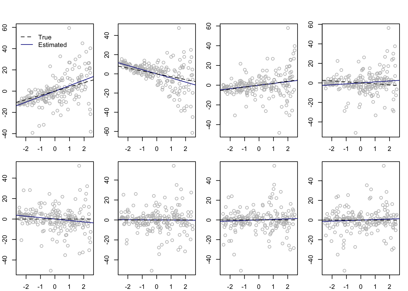
For each simulated data set, an \(n \times p\) design matrix \(\mathbf{X}= (x_{ij})_{1 \leq i \leq n, 1 \leq j \leq p}\) was generated such that each row was a realization of a random vector \(X \in \mathbb{R}^p\) of which each coordinate was Uniformly distributed on the interval \((-2,2)\) and where \(\mathbb{C}X = (\rho^{|i-j|})_{1 \leq i,j \leq p}\). We set \(p = 8\). Heteroscedasticity was imposed by setting \(\sigma_i^2 = 1/4 + (x_{i2} + 2.5)^2\) for \(i =1,\dots,n\), so that the variance of the error terms depended on the second covariate. Responses were generated with \(\boldsymbol{\beta}= (4,-3,2,-1,0,0,0,0)^T\) and \(\varepsilon_i \sim \mathcal{N}(0,\sigma_i^2)\) for \(i=1,\dots,n\). The contrast vector was set to \(\mathbf{c}= (0,1,0,0,0,0,0,0)^T\), so that confidence intervals were constructed for \(\mathbf{c}^T\boldsymbol{\beta}= \beta_2\). Over a range of sample sizes \(n\), we recorded the achieved coverage probabilities of the wild bootstrap confidence intervals based on \(Q_n\) and \(H_n\) as well as of the asymptotic confidence interval in Equation 39.1. For the sake of comparison, we also recorded the achieved coverage probabilities of the residual bootstrap confidence interval based on \(Q_n\) and \(T_n\) (from the previous section) as well as of the asymptotic confidence interval in Equation 38.2, even though these intervals are not suited to accommodate the heteroscedasticity in the error term variance.
Code
n <-200p <-8s <-4r <-0.7R <- r^abs(outer(1:8,1:8,"-"))P <-2*sin( R * pi /6)beta <-c(c(s:1)*(-1)^(s:1),rep(0,p-s))X <- (pnorm( matrix(rnorm(n*8),ncol =8) %*%chol(P)) - .5) *5sigma <-1/4+ (X[,2] +2.5)^2# make the error terms heteroscedasticerror <-rnorm(n,0,sigma)Y <-drop(X %*% beta) + errorbeta_hat <-solve( t(X) %*% X) %*%t(X) %*% YYY <-matrix(NA,n,p)for( j in1:p){ YY[,j] <- Y - X[,-j] %*% beta_hat[-j]}par(mfrow =c(2,4), mar =c(2.1,2.1,1.1,1.1), oma =c(0,0,2,0))for(j in1:p){plot(YY[,j] ~ X[,j],col ="gray")abline(a =0, b = beta_hat[j], col =rgb(0,0,.545))abline(a =0, b = beta[j], lty =2)if(j ==1){ xpos <-grconvertX(.15,from="nfc",to="user") ypos <-grconvertY(.9,from="nfc",to="user")legend(x = xpos,y = ypos,legend =c("True","Estimated"),col =c(1,rgb(0,0,.545)),lty =c(2,1),bty ="n") }}
Figure 39.1: Least-squares estimates of linear effects with points \((x_{ij},Y_i - \sum_{k\neq j}x_{ik}\hat\beta_k)\), \(i=1,\dots,n\) plotted in panels \(j=1,\dots,8\) (numbered left to right, top to bottom). Heteroscedasticity is most apparent in the second panel.
Code
# residual bootstrap for a contrast in linear regression coefficientsrbootc <-function(X,Y,cc,B,alpha){# fit the least-squares estimator n <-nrow(X) p <-ncol(X) XtX_inv <-solve(t(X) %*% X) XtX_inv_Xt <- XtX_inv %*%t(X) b_hat <-as.numeric(XtX_inv_Xt %*% Y) Y_hat <- X %*% b_hat ctb_hat <-as.numeric(t(cc) %*% b_hat) e_hat <- Y - Y_hat sigma_hat <-sqrt(sum(e_hat^2)/(n-p)) sigma_c_hat <-as.numeric(sqrt(t(cc) %*% XtX_inv %*% cc * n) * sigma_hat)# Do bootstrap resampling e_star <-matrix(e_hat[sample(1:n,B*n,replace=TRUE)],n,B) e_star_hat <- e_star - X %*% XtX_inv_Xt %*% e_star sigma_hat_star <-sqrt(apply(e_star_hat^2,2,mean)) b_star_minus_b_hat <- XtX_inv_Xt %*% e_star# CI based on Qn Qn <-sqrt(n) *as.numeric(t(cc) %*% b_star_minus_b_hat) Q_qtls <-quantile(Qn,probs =c(alpha/2,1-alpha/2)) Qlo <- ctb_hat - Q_qtls[2] /sqrt(n) Qup <- ctb_hat - Q_qtls[1] /sqrt(n)# CI based on Tn Tn <-sqrt(n) *as.numeric(t(cc) %*% b_star_minus_b_hat) / sigma_hat_star T_qtls <-quantile(Tn,probs =c(alpha/2,1-alpha/2)) Tlo <- ctb_hat - T_qtls[2] * sigma_hat /sqrt(n) Tup <- ctb_hat - T_qtls[1] * sigma_hat /sqrt(n)# CI based on the asymptotic Normal approximation zval <-qnorm(1-alpha/2) zlo <- ctb_hat - zval * sigma_c_hat /sqrt(n) zup <- ctb_hat + zval * sigma_c_hat /sqrt(n) output <-list( Qlo = Qlo,Qup = Qup,Tlo = Tlo,Tup = Tup,zlo = zlo,zup = zup)return(output)}# wild bootstrap for a contrast in linear regression coefficientswbootc <-function(X,Y,cc,B,alpha,type="Mammen"){# fit the least-squares estimator n <-nrow(X) XtX_inv <-solve(t(X) %*% X) XtX_inv_Xt <- XtX_inv %*%t(X) b_hat <-as.numeric(XtX_inv_Xt %*% Y) Y_hat <-as.numeric(X %*% b_hat) ctb_hat <-as.numeric(t(cc) %*% b_hat) e_hat <- Y - Y_hat cc_XtX_inv_Xt <-as.numeric(t(cc) %*% XtX_inv_Xt)# we do not need to do expensive matrix multiplications sigma_c_hat <-sqrt(n) *sqrt(sum(cc_XtX_inv_Xt^2* e_hat^2))if(type =="Mammen"){# Wild bootstrap of Mammen d1 <-sqrt(3/4+sqrt(17)/12) d2 <-sqrt(3/4-sqrt(17)/12) U1 <- d1 +matrix(rnorm(n*B),B,n)/sqrt(2) U2 <- d2 +matrix(rnorm(n*B),B,n)/sqrt(2) e_star <-t(scale(U1*U2 - d1*d2, center =FALSE, scale =1/ e_hat)) } elseif( type =="Das"){# Wild bootstrap of Das G_star_cent_scaled <-matrix( 4* ( rbeta(n*B, shape1 =1/2, shape2 =3/2) -1/4 ), B, n ) e_star <-t(scale(G_star_cent_scaled,center =FALSE, scale =1/ e_hat)) } e_star_hat <- e_star - X %*% XtX_inv_Xt %*% e_star sigma_c_hat_star <-numeric(B)for(b in1:B){ sigma_c_hat_star[b] <-sqrt(n) *sqrt(sum(cc_XtX_inv_Xt^2* e_star_hat[,b]^2)) } b_star_minus_b_hat <- XtX_inv_Xt %*% e_star# CI based on Q_n: Qw <-sqrt(n) *drop(t(cc) %*% b_star_minus_b_hat) Qw_qtls <-quantile(Qw,probs =c(alpha/2,1-alpha/2)) Qlo <- ctb_hat - Qw_qtls[2] /sqrt(n) Qup <- ctb_hat - Qw_qtls[1] /sqrt(n)# CI based on H_n: Hw <-sqrt(n) *as.numeric(t(cc) %*% b_star_minus_b_hat) / sigma_c_hat_star Hw_qtls <-quantile(Hw,probs =c(alpha/2,1-alpha/2)) Hlo <- ctb_hat - Hw_qtls[2] * sigma_c_hat /sqrt(n) Hup <- ctb_hat - Hw_qtls[1] * sigma_c_hat /sqrt(n)# CI based on the asymptotic Normal approximation zval <-qnorm(1- alpha/2) zlo <- ctb_hat - zval * sigma_c_hat /sqrt(n) zup <- ctb_hat + zval * sigma_c_hat /sqrt(n) output <-list( Qlo = Qlo,Qup = Qup,Hlo = Hlo,Hup = Hup,zlo = zlo,zup = zup)return(output)}# run the simulationS <-500B <-500alpha <-0.05cc <-c(0,0,1,rep(0,p-3))ctb <-drop(t(cc) %*% beta)nn <-c(10,20,30,40,50,60,70,80,90,100)cvg_rbootQ <- cvg_rbootT <- cvg_asympT <-numeric(length(nn))cvg_wbootQ <- cvg_wbootH <- cvg_asympH <-numeric(length(nn))for(k in1:length(nn)){ n <- nn[k] cov_rbootQ <- cov_rbootT <- cov_asympT <-numeric(S) cov_wbootQ <- cov_wbootH <- cov_asympH <-numeric(S)for(s in1:S){# generate data X <- (pnorm( matrix(rnorm(n*8),ncol =8) %*%chol(P)) - .5) *5 sigma <-1/4+ (X[,2] +2.5)^2# make the error terms heteroscedastic error <-rnorm(n,0,sigma) Y <-drop(X %*% beta) + error# get residual and wild bootstrap confidence intervals for the contrast rboot_out <-rbootc(X,Y,cc,B,alpha) wboot_out <-wbootc(X,Y,cc,B,alpha) # type = "Mammen" and type = "Das" give very similar results# record coverage results cov_rbootQ[s] <- (rboot_out$Qlo < ctb) & (rboot_out$Qup > ctb) cov_rbootT[s] <- (rboot_out$Tlo < ctb) & (rboot_out$Tup > ctb) cov_asympT[s] <- (rboot_out$zlo < ctb) & (rboot_out$zup > ctb) cov_wbootQ[s] <- (wboot_out$Qlo < ctb) & (wboot_out$Qup > ctb) cov_wbootH[s] <- (wboot_out$Hlo < ctb) & (wboot_out$Hup > ctb) cov_asympH[s] <- (wboot_out$zlo < ctb) & (wboot_out$zup > ctb) } cvg_rbootQ[k] <-mean(cov_rbootQ) cvg_rbootT[k] <-mean(cov_rbootT) cvg_asympT[k] <-mean(cov_asympT) cvg_wbootQ[k] <-mean(cov_wbootQ) cvg_wbootH[k] <-mean(cov_wbootH) cvg_asympH[k] <-mean(cov_asympH)}table <-rbind(cvg_rbootQ, cvg_rbootT, cvg_asympT, cvg_wbootQ, cvg_wbootH, cvg_asympH)colnames(table) <-paste("n =", nn)rownames(table) <-c("Q (resid)", "T (resid)", "Asymp iid (19.2)","Q (wild)","H (wild)","Asymp het (20.1)")library(knitr)
Warning: package 'knitr' was built under R version 4.4.1
Code
kable(table,digits =2)
n = 10
n = 20
n = 30
n = 40
n = 50
n = 60
n = 70
n = 80
n = 90
n = 100
Q (resid)
0.52
0.83
0.88
0.91
0.94
0.94
0.96
0.94
0.94
0.95
T (resid)
0.98
0.98
0.97
0.96
0.97
0.98
0.98
0.97
0.97
0.95
Asymp iid (19.2)
0.82
0.94
0.93
0.95
0.97
0.97
0.97
0.96
0.96
0.96
Q (wild)
0.52
0.82
0.86
0.90
0.94
0.93
0.95
0.92
0.93
0.95
H (wild)
0.89
0.93
0.92
0.92
0.95
0.93
0.93
0.92
0.93
0.93
Asymp het (20.1)
0.50
0.81
0.85
0.89
0.93
0.92
0.94
0.92
0.93
0.93
Das, Debraj, Karl Gregory, and Soumendra Lahiri. 2019. “Perturbation Bootstrap in Adaptive Lasso.”The Annals of Statistics 47 (4): 2080–2116.
Mammen, Enno. 1993. “Bootstrap and Wild Bootstrap for High Dimensional Linear Models.”The Annals of Statistics, 255–85.
White, Halbert. 1980. “A Heteroskedasticity-Consistent Covariance Matrix Estimator and a Direct Test for Heteroskedasticity.”Econometrica: Journal of the Econometric Society, 817–38.